Submitted:
07 June 2024
Posted:
10 June 2024
You are already at the latest version
Abstract
The savings behavior of individuals has been a topic of both macroeconomic and policy importance throughout history. Theoretical and empirical research offers strong evidence that savings are the result of a number of demographic and economic factors working together to produce long-term, sustainable economic growth. This study therefore looked at how domestic savings affected South Africa's economic growth between 1970 and 2022. The ARDL framework was used to analyze data that came from the World Bank and the South African Reserve Bank. The results of the study demonstrate that corporate savings have a major effect on economic growth, especially over the long term. When corporate savings rise by 1%, the economy expands by 3.12%. On the other hand, savings by the government and the general public, especially in the long run, have no appreciable impact on economic growth. Given that domestic savings mobilization is the most suitable channel for financing capital accumulation to support economic growth and development, the study suggests reviewing current policies to encourage domestic savings mobilization.
Keywords:
corporate savings
; economic growth
; government savings
1. Introduction
One of the main tenets of growth theory has long been the importance of savings in economic development. This theory draws its foundation from traditional research, including the Endogenous Growth Models, Classical Economic Growth Models, Harrod-Domar Growth Model, and Solow Growth Model, among others. According to these studies, savings are the primary driver of economic expansion and growth (Chakraborty, 2023). According to Ackah & Lambon-Quayefio (2023), a country with a low domestic saving rate will continue to grow modestly. This is supported by the Harrod Domer model, which postulated that savings are essential for economic growth. Moreover, this kind of saving is very important. Osei & Kim (2020) contend that a country’s economy will suffer if it relies primarily on foreign resources to finance investments, making it more vulnerable to external shocks. Thus, to ensure long-term sustainable economic growth, this is a significant issue that requires careful understanding and attention.
The causal relationship between savings and economic growth has been the subject of numerous studies, most of which have focused on Asia and Latin America with little to no reporting from countries in Sub-Saharan Africa (Adedokun, Falayi & Adeleke, 2020). The majority of the research done in this field has focused on the connection between overall savings and economic growth. The best conditions for conducting empirical research to ascertain the effects of various domestic savings sources on economic growth are provided by African countries such as South Africa, which have strong banking sectors and financial markets (Wyk & Kapingura, 2021). South Africa, which has one of the biggest economies in Africa, has recently come under fire for having a low savings culture and slow rates of economic growth. Over the past ten years, the country’s total savings have dropped to an all-time low. The average gross domestic savings rate between 1995 and 2007 was only 15%, down from over 25% during the 1970s and late 1980s, when compared to comparable level nations like Malaysia, which averages between 25 and 43% (Eyraud, 2009; Tendengu, Kapingura & Tsegaye, 2022).
The low domestic savings rate of the nation is preventing faster economic growth, which is very important in mobilizing savings to create effective capital for economic growth, according to Šubová, Buleca, Affuso & Mixon (2023) and Govdeli (2022). This basically relates to the notion that in order to finance sufficient investments for economic growth, any economy must either generate enough savings or, alternatively, borrow from sources outside its borders. Foreign borrowing, however, isn’t always the best option because it exposes countries to a variety of additional risks, including negative effects on their balance of payments and fluctuations in foreign exchange rates (Osei & Kim, 2020). But since the end of the apartheid era and South Africa’s economic isolation from the rest of the world, the country has consistently seen a decline in gross domestic savings rates. During this time, the country has borrowed more money to finance its investment projects and has also seen a rise in foreign direct investment. Domestic savings are no longer the main source of funding as a result. Government, corporate, and household savings make up the three components of total domestic savings. These three categories require more attention in order to raise savings levels and create the best possible policy responses for domestic savings in South Africa.
There is no doubt that there are several flaws in the growing empirical literature on the savings-growth relationship that call for more investigation. Studies such as Arestis & Demetriades (1997) and Demetriades & Hussien (1996), for example, have ignored the differences in the institutional and economic features of the developed and developing economies in favor of cross-sectional panel data from both economies. In addition, some of these studies’ other characteristics include their brief time span and improper use of econometric techniques. This work aims to make several contributions to the body of current empirical literature. Using the instantaneous causality econometric technique, we first reexamine the short- and long-run relationships under the ARDL framework, assessing the validity of the widely used Granger and Toda-Yamamoto causality tests. Second, we apply the aforementioned methods to comparatively longer time series data from 1970 to 2022 in comparison to the cross-sectional studies, and the robustness check is assessed using the Innovation Outlier model for outlier detection, CUSUM, and the CUSUM of Squares. Lastly, the study sought to test three hypotheses: that is, (household savings has no influences on economic growth in South Africa; corporate savings has no influences on economic growth in South Africa; and government savings has no influences economic growth in South Africa.
This paper’s structure is set up as follows. A thorough analysis of the theoretical and empirical research on domestic savings and economic growth is provided in Section 2. Our data sources and model specification are described in Section 3. Results, debates, conclusions, and policy recommendations are presented in Section 4 and Section 5.
2. Literature Review
2.1. Theoretical Review
Higher savings rates are thought to accelerate capital accumulation and economic growth, according to the majority of growth theories. Economic theorists such as Ricardo and Robert Torrens were influenced by the Corn Model , which is the source of the original theory surrounding the laws of capital accumulation and economic growth. These economists postulated that in an environment of unrestricted competition, all economic surplus would be invested or saved, and that the surplus rate would supply the general economic growth rate as well as the rate of profit.
But the theoretical underpinnings of the relationship between savings and economic growth date back to the early growth models of Domar (1946) and Harrod (1939), which took capital—rather than labor—as the output-limiting factor. According to the Harrod-Domar model, a continuous, proportionate increase in output is caused by surplus capital . The incremental capital output ratio, or , is this; a high indicates less productive technology: . The savings function, , is expressed as the product of the rate of saving and output (i.e., ), and the investment function, , is equivalent to . The aggregate productive function is represented by , which is equal to . According to the model, the economy’s growth rate will rise in tandem with the savings rate (s) and fall in tandem with .
The Harrod Domar model’s inability to account for labor substitutions, declining returns on capital, or technological advancements is one of its drawbacks. Neo-classical economist Robert Solow’s (1956) well-known growth model, which aims to address some of the shortcomings of the Harrod-Domar model, allows for the substitution of labor for capital and decreases marginal returns to capital. Ultimately, Solow concludes that growth eventually slows down, but economies with higher savings rates have higher steady incomes. Here is how the model is defined: is the economy’s aggregate production, where is the TPF. is another way to express the production function because f has continuous proceeds to gauge. The economic growth rate of output is given by the model’s condensed form as follows:
where is the capital price and = Share of capital in total cost. The rate of technical change is expressed as or TFP growth, and the labor stake in total cost is expressed as and =price of labor. On the other hand, factor deepening is represented by = and the rate of factor accumulation by = . The unresolved leftover from economic growth is the rate of technological change, or . This can be calculated as follows:
On the other hand, authors like Adam Smith pursued to find the origins of the motivation by people to accumulate capital. Kurz & Salvadori (2002) noted that in Adam Smith’s view, the growth process was endogenous. He highlighted the importance of capital accumulation on labour productivity. A distinctive view of the classical methodology was that production involves labour and that capital accumulation propels this process forward and, in the process, creates new markets, expands existing markets, while it increases demand and supply, to ultimately result in economic growth and social development of nations. As a result, due to importance of domestic saving to investment, there is need for deeper understanding of the relationship between domestic saving and economic growth.
2.2. Empirical Review
Around the world, a plethora of empirical research has been conducted on the connection between domestic savings and economic growth. This is because many countries, both developed and developing, have seen a decline in their rates of savings and economic growth (Tendengu et al., 2022). The role of investments through savings, which have an impact on economic growth and development, has also been a driving force behind the ongoing investigation of causality. The main goal of recent empirical research on the connection between domestic savings and economic growth in South Africa was to analyze the growth-savings hypothesis from the standpoint of total domestic savings.
Amusa (2013) and Getachew (2015) conducted separate studies to examine how various types of domestic savings contribute to South Africa’s economic expansion. Amusa (2013), for example, used a co-integration analysis within a multivariate framework to ascertain how government, corporate, and household savings affected South Africa’s economic growth. Understanding the contributions of the various types of domestic savings to economic growth is crucial, according to Amusa (2013). The study evaluated the short- and long-term effects of the various forms of domestic savings on economic growth using the Auto Regressive Distributed Lag (ARDL) approach to co-integration. The findings show that while household and government savings have no discernible long-term effects on economic growth, corporate savings have a considerable impact both in the short and long terms. Further analyses were motivated by the research conducted by Amusa (2013) and Getachew (2015), since policies that can boost domestic savings rates and aid in the creation of government policies are desperately needed.
For the BRICS nations, Chakraborty (2023) examined the causal relationship between domestic savings and economic growth. The short- and long-term relationships between savings and economic growth have been studied using the panel ARDL model. The study’s findings indicate that gross domestic savings plays a major role in explaining economic growth over the long and short terms. Furthermore, the results of both causality tests support the idea that savings and economic growth in the BRICS countries are causally related in both directions. Similar to this, Sellami et al. (2020) used ARDL to examine the short- and long-term effects of domestic saving on Algeria’s economic growth from 1980 to 2018. In Algeria’s case, where saving rates are high and strongly correlated with economic growth, the findings show the substantial short- and long-term effects of saving on economic growth. Granger’s causality test and the Toda-Yamamoto procedure were used by Đidelija (2021) to examine the direction and strength of savings causality and economic growth in Bosnia and Herzegovina. Granger’s causality test results showed that there is no causal relationship between the elements of private savings and economic growth.
In Kosovo, Ribaj & Mexhuani (2021) looked at the relationship between savings and economic growth from 2010 to 2017. The results of the regression analysis demonstrated that deposits significantly boost Kosovo’s economic growth because savings encourage investment, output, and employment, all of which led to more sustained economic growth. Their research also demonstrates that nations with high national savings rates are less reliant on foreign direct investment, which significantly reduces the risk associated with volatile foreign direct investment. Nguyen & Nguyen (2017) used the ARDL bound testing approach to examine the short- and long-term effects of domestic savings on Vietnam’s economic growth between 1986 and 2015, taking dependency ratio and domestic investment into consideration. According to the short-run estimates, the dependency ratio, domestic savings, and domestic investment have no bearing on economic growth. According to long-term estimates, Vietnam’s economic growth is primarily driven by domestic savings and investment, with the dependency ratio having a detrimental effect on growth.
The literature review indicates that while some empirical studies have been conducted abroad, there is still a dearth of literature specifically about South Africa, which calls for further research. Additionally, it has been noted that the literature is unsettling and that the findings of different empirical investigations appear to be inconsistent. In order to add to the empirical literature of the nation, this study examined the effects of the various sectors of domestic savings on economic growth in South Africa.
3. Methodology
3.1. Data Source
Depending on the data’s availability, annual time series data covering the years 1970–2022 were used in this study. Fedderke & Liu (2015) claim that because countries exhibit greater levels of heterogeneity, time series data may be more trustworthy than panel data. The World Bank’s World Development Indicators provided the economic growth data, which was proxied by GDP. The South African Reserve Bank provided the information on savings for households, governments, and corporations.
3.2. Description of Study Variables
Household savings (HHS), government savings (GOS), corporate savings (COS), and gross domestic product are the study’s variables of interest. After direct taxes are paid, the HHS can be characterized as a portion of current income that is neither transferred nor consumed as part of household current consumption (Xu, 2023). According to Sisay (2023), household savings include current outlays made in the form of a decrease in debt, such as capital repayment on loans for consumer durables and housing. Typically, HHS savings are separated into contractual and discretionary savings. Nonetheless, the distinction between the two forms of HHS is not very important for the purposes of this investigation.
The total of retained taxes and public enterprise profits, along with any receipts that the government does not allocate to current spending, is known as the GOS (Xu, 2023). Prinsloo (2000) states that the estimate of COS is the total of the gross operating surpluses of businesses less the net dividends, interest, rent, and royalties that these businesses owe to other economic sectors and the global community, less direct income and wealth taxes, and less other net transfer payments to the general public, households, and other businesses. As a result, the model will take the following form and incorporate the various forms of domestic savings in the economy:
where is the dependent variable (Gross Domestic Product) at time ; is household savings at time ; government savings is at time ; is corporate savings at time ; and is the random error.
Lastly, the total value of all goods and services produced in a nation in a given year can be defined as the GDP (OECD, 2016). Although there are a number of ways to gauge a nation’s economic growth, real GDP is the most widely used indicator. Since GDP serves as a proxy for economic growth, it is critical to calculate how the various sectors of domestic savings affect growth in the context of South Africa. Thus, an estimate of the GDP was as follows:
where is GDP at time ; is private consumption at time ; is gross investment at time ; is government investment at time ; is government spending at time ; is exports at time ; is imports at time . In gross domestic product, “gross” means that GDP measures production regardless of the various uses to which the product can be put. Table 1 provides study variables, their description and data source.
3.3. Unit Root Test
It is crucial to check for non-stationarity because the data contains time elements. Non-stationarity variables can lead to spurious regression results and increase the confidence intervals for estimated coefficients, according to Najarzadeh et al. (2014). Testing for stationarity in data is therefore essential. The unit root test with structural breaks was used to determine whether the time series data was stationary. According to Verma (2007), institutional arrangements, policy changes, regime shifts, and economic crises all cause structural change in a variety of time series. Verma (2007), the author, also emphasizes how structural change has gained significance recently in the analysis of macroeconomic time series data.
Perron (1989, 1997) asserts that results may be skewed in favor of the non-stationarity hypothesis when such structural changes occur during data collection and are not permitted. Therefore, Perron and Vogelsang (1992) and Perron (1997) proposed the Additive Outlier model for instantaneous structural change and the Innovational Outlier model (IOM) for gradual structural change in order to allow for various forms of structural breaks to occur. The intercept (I0M1) can change gradually in the model, but the incline of the trend function and the intercept can change steadily in IOM2.
The time of the break is indicated by , while () which is unknown, = 1 where it is greater than and 0 (Zero) alternatively, is a general process while is the assumed residual term. According to Perron (1997) the unit root – null hypothesis was rejected when the outright value of the -statistic for test than equivalent critical value.
The IOM model will be used in this study because South Africa underwent a gradual structural change. The three variables were tested for stationarity and non-stationarity using the IOM model. It is well known that the stationarity test under structural change has minimal impact and may lead to a different order of variable integration (Verma, 2007). Therefore, the co-integration ARDL method was used in the study to allow for mixed order integration and a long-run relationship between variables.
3.4. Motivation to Use ARDL Model
A variety of techniques are available to test co-integration; these include the Gregory-Hansen, Johansen-Juselius, and Engele-Granger models. Research on the impact of domestic savings in Vietnam by Kim & Nguyen (2017) noted that the ARDL approach, which was first developed by Pesaran, Shin, & Smith (1995, 1998) and then refined by Pesaran, Shin, & Smith (2001), has become extremely popular in recent years for a variety of reasons. Pesaran, Shin, & Smith (1996), Brooks (2014), and Paul (2014) all concur, stating that the ARDL approach has several benefits over conventional statistical techniques for evaluating con-integration and short- to long-term relationships.
According to Pesaran et al. (2001), unlike the Johansen-Juselius model, the ARDL does not require that variables be in the same order. Furthermore, it is possible to estimate both the long- and short-term relationships at the same time, and calculating long-run relations doesn’t require changing the data in any way. As a result, the model can be applied with ease to large samples of data and performs well with both small samples. Additionally, the dependent and explanatory variables are distinguished by the model. According to Hendrix, Pagan, & Sargan (1984), the ARDL approach is an attempt to match an actual quantified econometric model with the process of producing anonymous data. This study employed the ARDL method because of the advantages that have been suggested.
3.5. Model Specification
This study will use the ARDL bound testing approach in order to ascertain the effect of domestic savings on economic growth. In recent years, the suggested ARDL model has gained a lot of popularity. The model ARDL can be expressed as follows:
In the equation, the parameters capture the coefficients of the short-run dynamic, and
are the long-run-multipliers, while denotes the first difference operator denotes one-period lag, denotes the sum of denotes the sum of . The bounds test approach requires examining the null hypothesis of an absent conditional or ‘no conditional’ relationship using a joint significance test, the -test, of the lagged levels of the variables. Taking GDP as the dependent variable, the null hypothesis of no co-integration is
against the alternative hypothesis (. This is denoted by . The null and alternative hypotheses are evaluated on the basis of estimated standard -statistic.
Narayan (2005) computes the critical values for small samples ranging from 30-80 observations, which is applicable to this study. The critical value bounds hold for all classifications of regressors that are into purely , purely or mutually co-integrated (Narayan & Singh, 2007). Determination of co-integration rests on the -statistics and the upper and lower bounds. If the computed -statistic falls outside the upper bound, the null hypothesis of no co-integration is rejected. If the computed -statistics falls below the lower bound, the conclusion that the null hypothesis cannot be rejected is reached, and if the computed -statistics falls within the critical value band, the result of inference is inconclusive.
4. Results and Discussion
4.1. Descriptive Statistics
The descriptive statistics for each of the individual variables are shown in real terms in Table 2 above. The following are the Jarque-Bera statistics and their corresponding -values: 4.665 (0.097), 28.788 (0.000), 12.012 (0.002), and 5.068 (0.079). Given that all of the variables have a normal distribution with a 10% significance level, the results are indicative. Given that the standard deviation captures the trend in the data, it appears to be very high for each variable.
4.2. Correlation Analysis
A correlation matrix, shown in Table 3 above, provides an overview of the correlation. With the exception of GDP and government spending, which have a very weak positive correlation (0.265), all the variables have a very weak negative correlation (ranging from -0.008 to -0.270). As a result, the model retains all of the variables.
4.3. Diagnostics Test
4.3.1. Unit Root Testing
The findings of the unit root tests for the variables under investigation are shown in Table 4. Since the -values of 0.887, which is greater than 0.05, and the absolute value of the Augmented Dickey-Fuller test statistic value is 0.47, which is less than 2.92, GDP has a unit root. But with an ADF of 4.467 at the first deference, the unit root vanishes at the -values of 0.0003, greater than 2.94 at the 0.05 significance level. Since the Augmented Dickey-Fuller test statistic value is 4.47, which is greater than 2.94 and has a -values of 0.001, which is less than 0.05, HS do not have a unit root. Conversely, the results show that COS have a unit root because the -values is greater than 0.05 and the absolute value of the Augmented Dickey-Fuller test statistic value is 2.33, which is less than 2.92. At the first deference, the unit root vanishes with an ADF of 6.7044, indicating a p-value of 0.0000 and a significance level of greater than 2.92 at 0.05.
Given that the p-value of 1.000 is greater than 0.05 and the absolute value of the Augmented Dickey-Fuller test statistic value is 2.634, which is less than 2.93, GS have a unit root. At the 0.05 significance level, the unit root vanishes with an ADF of 3.888, which is higher than 2.94 at the first deference. Before performing additional analysis, COS and GOS should be respected due to the unit root present in the manner indicated by the results.
4.3.2. Serial Correlation
To test the alternative of serial correlation against the null hypothesis of no serial correlation, the Breusch-Godfrey LM test with four lags length was conducted. These are the outcomes in Table 5.
With an F-statistic of 1. and a p-value of 1.011 which was more than 5% significant level, the null hypothesis failed to be rejected, and this means that there was no serial correlation of the error term.
4.3.3. Heteroscedasticity Test
The white test, also known as the Breusch-Pagan test for heteroskedasticity, provides a definitive assessment of whether the error terms’ variance was constant. The results of testing the alternative hypothesis—that the error terms are heteroscedastic—as well as the null hypothesis—that there is no homoscedasticity of the error terms—are presented.
The result in Table 6 shows that -statistic of 1.37 and a -value of 0.48 which was more than 5% significant level, so we fail to reject the null hypothesis and this confirmed that there was no heteroskedasticity of the error term.
4.4. Empirical Results
However, the proper lag specifications had to be obtained before the ARDL co-integrations test could be performed. Table 7 presents the outcomes.
The ARDL model estimation requires the optimal lag length requirements needed to account for the autoregressive nature of time series data. The findings indicate that 1 was the optimal lag length for GDP (AIC) based on the Akaike criteria. It is crucial to stress that this lag length was also determined by the two other information criteria. The two other measures, the log likelihood ratio (LR) and the final prediction error (FPE), concur on the same lag length. Based on the aforementioned, the optimal lag structure for HHS is 2, as determined by taking into account all lag length determination criteria. Meanwhile, the optimal lag for COS is 0, as determined by examining the AIC, and the optimal lag for GOS is 2, as determined by examining the AIC. The ARDL model is expressed as follows:
The null hypothesis was evaluated, denoted as Ho in this test because there isn’t a co-integrating equation. The null hypothesis asserts that Ho is false otherwise. As a result, the ARDL bound test in Table 8 indicates that co-integration exists in the given data. and are the two bounds in this case. The upper bound is , and the lower bound is . The value of the -statistic indicates the co-integration of the variables. We conclude that there is no co-integration among the variables if the value is less than the critical bound values. We reject the null hypothesis since it is evident that the computed -statistic (11.50) is higher than the crucial value for the upper bound . This suggests that there isn’t a long-term

Table 8.
Autoregressive Distributed Lag Bound Test Results.
| Test Statistic | Value | K |
|---|---|---|
| F-statistic | 11.507 | 3 |
| Critical Value Bounds | ||
| Significance | Bound | Bound |
| 10% | 2.45 | 3.52 |
| 5% | 2.86 | 4.01 |
| 2.5% | 3.25 | 4.49 |
| 1% | 3.74 | 5.06 |
Source: Authors’ computation.
Table 9.
ARDL Model Results.
| Variable | Coefficient | Standard Error | t-Statistic | Prob. |
|---|---|---|---|---|
| Constants | 0.005 | 0.002 | 2.725 | 0.009 |
| 0.419 | 0.148 | 2.823 | 0.007 | |
| 1.031 | 0.001 | 865.674 | 0.000 | |
| -1.464 | 0.153 | -9.548 | 0.000 | |
| 0.433 | 0.153 | 2.823 | 0.007 | |
| 0.0001 | 6.69E-05 | 1.776 | 0.083 | |
| -0.0002 | 8.00E-05 | -2.256 | 0.030 | |
| 1.33E-05 | 9.23E-05 | 0.144 | 0.886 | |
| -7.49E-05 | 0.0001 | -0.742 | 0.462 |
Note: Adjusted- =0.999; Prob(F-statistic) = 0.000; S.E. of regression = 0.0001. Source: Authors’ computation
Table 10.
Estimation of Co-integrating vector (The long-run ARDL equation).
| Variable | Coefficient | Standard Error | t-Statistic | p-value |
|---|---|---|---|---|
| 4.597 | 1.124 | 4.087 | 0.000 | |
| -0.179 | 0.182 | -0.984 | 0.031 | |
| -0.668 | 0.258 | -2.586 | 0.014 | |
| 0.829 | 0.568 | 1.458 | 0.053 | |
| Constant | -17.896 | 6.701 | -2.670 | 0.011 |
Source: Authors’ computation.
The ARDL model is as per the results is given as:
The long-run co-integration model is given as:
The co-integration of variables is indicated by the -statistic value. It was concluded that there is no co-integration among the variables if the -value is less than the critical bound values. The regression equation’s goodness of fit, or how well the independent variable has been explained by the equation, is gauged by the coefficient of determination (). Since all of the explanatory variables together account for 99.9% of the changes in the dependent variable, the in this case is 0.999, or roughly 99.9%.
4.5. Discussion of Results
This study’s main goal was to investigate how different domestic savings domains affect economic growth. According to the analysis, economic growth is influenced by all spheres, including household, government, and COS. There are both short- and long-term relationships between the variables, according to the bounds test results. The ARDL model for co-integration was used to further test the relationship and found that COS had the largest influence on economic growth. It is noteworthy to emphasize that these results align with the various growth theories discussed in the theoretical review. The analysis’s findings help us determine where more attention should be paid in order to boost domestic savings, which can then encourage larger investments and accelerate economic growth. Only when there are larger savings can there be more investment. The analysis comes to the conclusion that lower government spending raises national savings and spurs investment in the private sector. Higher investment has the potential to increase both the economy’s potential and actual output levels over time.
Additional research has been done to examine the impact of savings on economic expansion (Shaw, 1973; McKinnon, 1973; Sajid & Sarfraz, 2008). The studies’ conclusions showed that although there is a strong correlation between saving and economic growth, there has been ongoing discussion among academics regarding which way the two variables are causally related. According to Solow (1956), higher savings usually come before and after stronger economic growth. According to a study by Sinha (1998), increasing saving leads to higher capital formation, which helps to explain the role that savings play in economic growth. The study also demonstrated a rise in investment, which boosted the expansion of the economy’s national output. Following Solow’s assertions, a number of academics—including Jappelli & Pagano (1994), Alguacil, Cuadros, & Orts (2002)—observed that greater savings growth comes before greater economic growth. Further research conducted by academics such as Gavin, Hausmann, & Talvi (1997), Sinha (1998), and Agarwal (2001) showed that increased economic growth precedes and leads to increased savings.
It should be noted that the results of this research lend support to a number of traditional growth models, including Romer (1986) and Solow (1956). Generally speaking, these growth models imply that greater savings lead to higher growth by expanding the domestic capital pool. As a result, physical capital accumulates more quickly, which is thought to be the primary driver of economic growth. Thus, it can be concluded that domestic savings are a crucial signpost and prerequisite for greater rates of economic expansion. Additional research conducted by a variety of economists, including Caroll & Well (1993), Sinha (1998), and Anoruo & Ahmad (2001), has demonstrated that the relationship between savings and growth is likely overstated and lends credence to the theory that savings drives growth rather than the other way around.
4.5.1. Hypothesis 1: HHS Has No Influences on Economic Growth in South Africa
The study aimed to investigate the first hypothesis, which stated that HSS had no bearing on South Africa’s economic growth. In the long-run growth savings equation, the HSS coefficient was 2.45%, and at the 95% confidence level, the p-value was 0.031, indicating significance. A 1% increase in the HHS will eventually result in a 2.45% increase in GDP, holding all other variables constant. The contribution of household savings to economic growth is confirmed by this study. This outcome agrees with those of Ribaj & Mexhuani (2021), Siaw, Enning & Pickson (2017), and Chakraborty (2023). For example, Chakraborty (2023) used ARDL to study the functional interrelationship between savings and economic growth in the BRICS countries and discovered that gross domestic savings significantly explains economic growth both in the short and long runs. This is so that savings can increase employment, investment, and production, all of which lead to more sustained economic growth.
4.5.2. Hypothesis 2: COS Has No Influences on Economic Growth in South Africa
This study aimed to investigate the second hypothesis, which stated that cooperative savings had no bearing on South Africa’s economic expansion. With a p-value of 0.014, the COS coefficient in the long-run growth savings equation was 3.17%, indicating statistical significance at a 95% confidence level. In the long run, a 1% increase in cooperative savings raises GDP by 3.17% while keeping all other variables constant. This study demonstrates that collective savings promote economic expansion. This outcome agrees with what Ribaj & Mexhuani (2021) found. Using Johansen cointegration tests, Ribaj & Mexhuani (2021) examined the relationship between savings and economic growth from 2010 to 2017 and discovered that corporate savings have a direct positive impact on investment, which in turn helps Kosovo’s economy grow. According to a study by Adam, Musah & Ibrahim, (2017), there is a positive and statistically significant correlation between COS and real GDP growth. According to the study’s findings, a 100% increase in GDP corresponds to an 18.5% increase in COS.
Although minimal research has examined the influence of different domestic savings domains on GDP, the observation that COS has emerged as the predominant factor is in line with the conclusions of previous studies conducted in South African contexts by Aron & Muellbauer (2000), Prinsloo (2000), and Guma & Bonga (2016). It should be mentioned that Abu (2010) used Granger causality and co-integration analyses to examine the relationship between savings and economic growth in Nigeria using data spanning from 1970 to 2007. The variables—economic growth and savings—are cointegrated, according to the Johansen co-integration test, which also revealed that COS had a substantially greater impact on GDP than both household and GOS. In addition, the study found that the two variables are in a long-term equilibrium. Furthermore, the Granger causality test indicated that, generally speaking, causality flows from economic growth to saving based on the study’s findings. In general, this suggests that saving comes from Granger and economic growth comes first.
4.5.3. Hypothesis 3: GOS Has No Influences Economic Growth in South Africa
This study aimed to investigate the third hypothesis, which stated that GOS had no bearing on South Africa’s economic growth. With a p-value of 0.538, the long-run growth savings equation’s GOS coefficient of 0.66% was statistically significant at a 90% confidence level. Over time, a 1% increase in the GOS raises GDP by 0.66%, assuming all other variables stay the same. This indicates that GOS plays a role in improving economic growth. The study’s conclusions also showed that a 1% increase in GOS over time raises GDP by 0.6687 percent. Numerous comparable studies have produced contradictory results. According to the study’s findings, GOS showed the least amount of response to variations in GDP growth over time. The researchers claim that the general lack of financial discipline played a role in this. An increase in long-term economic growth requires higher investment in the OECD economies in order to be attained; otherwise, faster growth can generate unsustainable pressure on the resources, according to a study conducted by Herd (1989) about some of the main effects of increased government saving on the economy.
4.6. Model Stability Test
- (a)
- The outlier detection Innovation Outlier model (IOM)
An initial impact that persists over subsequent observations is what defines an IO. The ARDL model’s plot against each independent variable is depicted in the graphs shown in Figure 1 below. There are a few true outliers in the model, but not enough to significantly alter it because of the large enough sample size.
Figure 1.
Stationarity Test. Source: Authors’ computation.
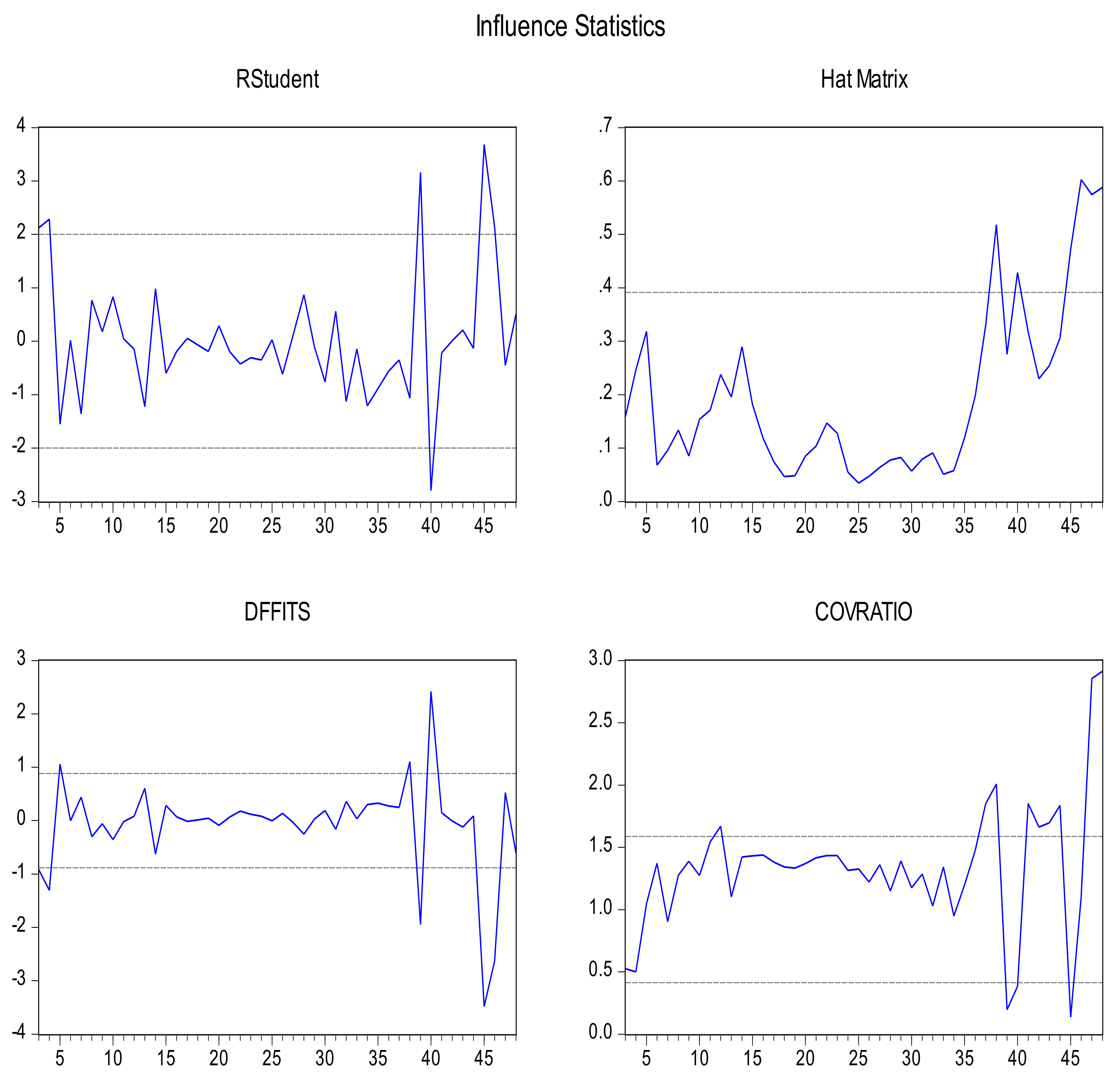
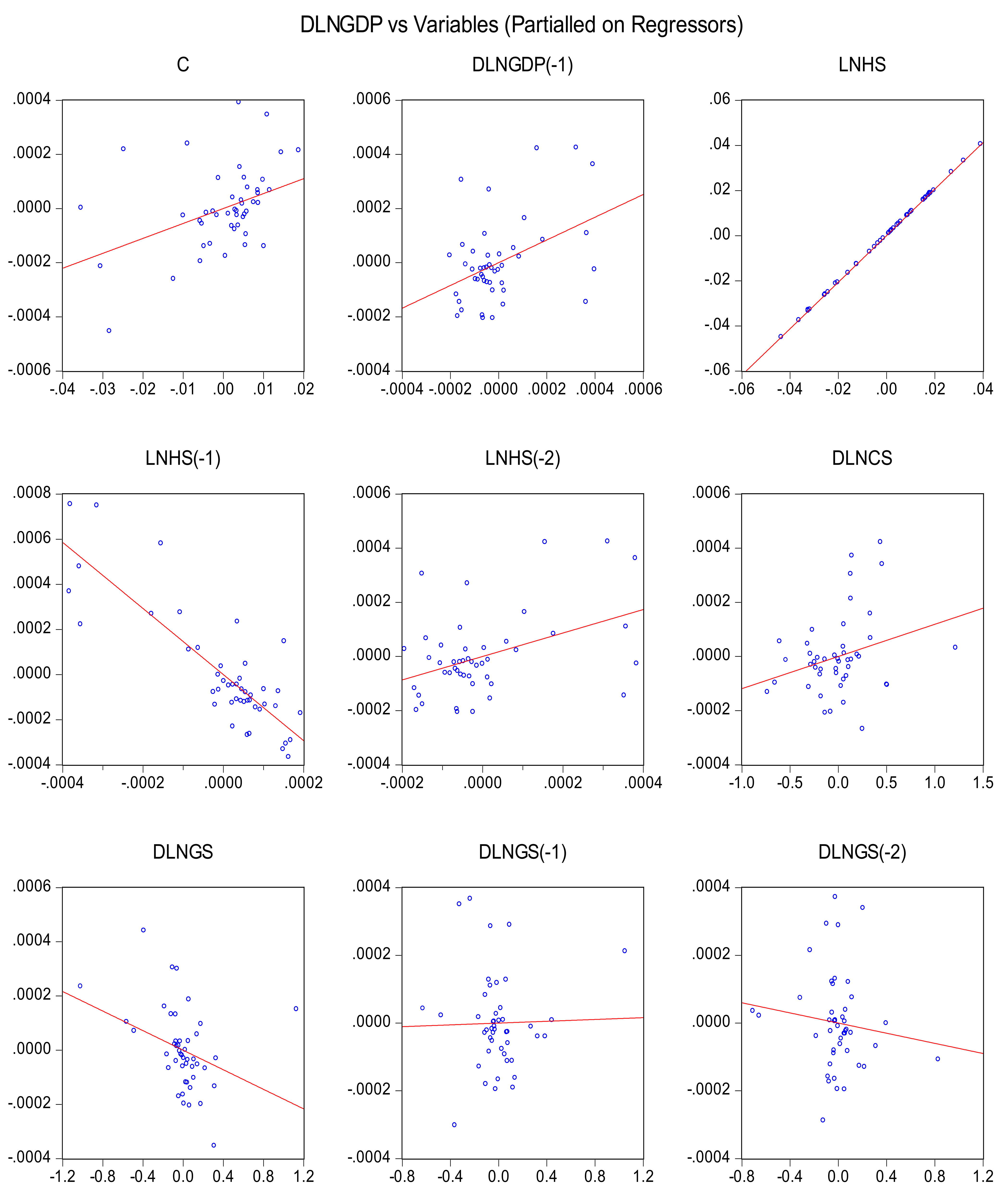
Figure 2.
Plot Against Variables. Source: Authors’ computation.
- (b)
- CUSUM and the CUSUM of Squares
Figure 3.
The CUSUM and CUSUM of square charts. Source: Authors’ computation.
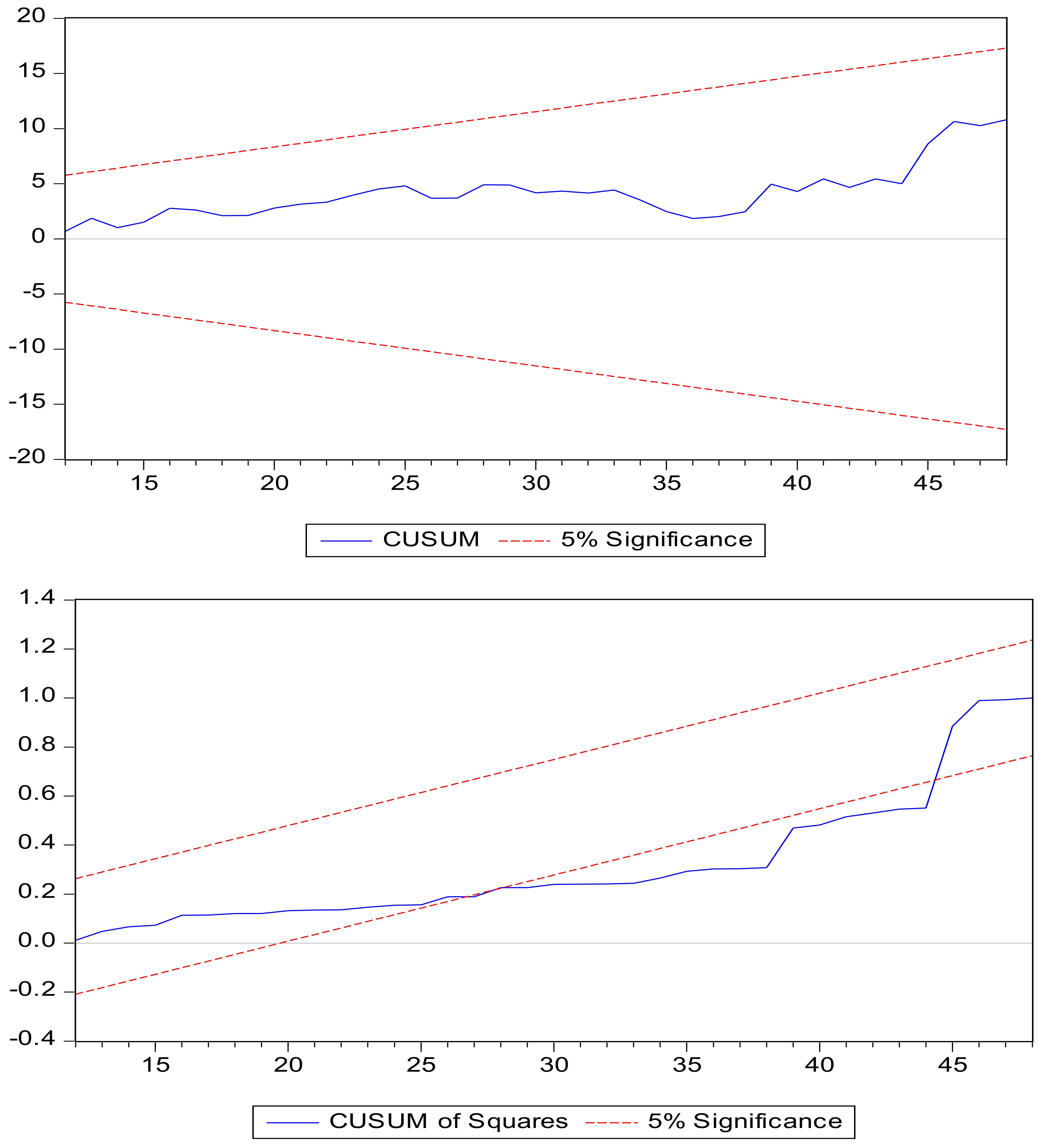
The stability of this model has been tested in this study using the CUSUM and the CUSUM of squares chats. The boundaries of the 5% significance level are shown in both graphs by the red dotted lines. Given that the blue line, which represents the model, stays inside the red dotted lines, it is evident that the model satisfies the CUSUM Test condition at the 5% significance level. But because the blue line crosses outside, the model fails the CUSUM of squares test. As a consequence of the CUSUM statistic remaining within the 5% critical bound, the Stability test results demonstrate that the estimated ARDL long-run model was both structurally and dynamically stable.
5. Conclusion and Policy Recommendation
5.1. Conclusion
The ongoing discussion about economic growth in South Africa requires an understanding of how to raise domestic savings rates. Because of its current excessive reliance on foreign funding, South Africa needs to increase its domestic savings rates in order to provide the foundation for future economic growth. The ARDL bond test was employed in the study to investigate how domestic savings affect economic growth. The ARDL model’s diagnostic tests were sufficient. The GOS coefficient was significant at 90% confidence level, while the HS and COS coefficients were significant at 95% and 90%, respectively. The results from the empirical analysis of the relations between domestic savings and economic growth in South Africa reflect the importance of savings to the country’s growth. The fact that COS have the most significant impact on economic growth is not much of a surprise as household and GOS contributes minimally to national savings. The CUSUM stability test revealed some shocks with the CUSUM of square test, but the model also passed stability diagnostics. With an R2 of 0.999, the model derived from this research validates savings as the primary driver of economic growth. The significance of savings for the growth of the nation is demonstrated by the findings of the empirical investigation of the relationships between domestic savings and economic growth in South Africa. Given that household and GOS contributions to national savings are negligible, it is not surprising that COS have the greatest influence on economic growth.
5.2. Policy Recommendation
The study’s conclusions highlight the important contributions that HHS and corporations make to economic growth. The study’s conclusions also show that, by accelerating various types of investments within the economy, total domestic savings contribute significantly to economic growth and development. Various measures ought to be implemented in order to guarantee a rise in household and COS. Gaining an understanding of how to increase domestic savings is essential to the growth discussion. Higher levels can be attained by implementing policies that permit corporations to hold onto their earnings rather than paying out dividends to households. A rise in HHS is very helpful to the national economy in fostering highly sustainable prosperity while also playing a significant role in ensuring that families have more financial security.
The current savings incentives, such as annuity savings plans and tax-free savings schemes, should be preserved and made simpler by policymakers. In addition, the entire restructuring process is focused on optimizing savings—both overall and within the groups that are currently least able to save. Those who are not covered by workplace plans ought to be included in this. Furthermore, it should be acknowledged that workplace payroll savings plans are the primary factor behind the accumulation of assets among South Africa’s working class. It should be mentioned that these plans always function best when they are set up to be completely “automatic” and when the deferral rates are highly appropriate. Similarly, working households can contribute to this process by increasing their savings and adopting a more disciplined spending approach.
Policymakers must collaborate with other stakeholders. Employers, financial service providers, and working households themselves ought to be included in the process of identifying the most effective strategies for increasing investments and savings. In the long run, this would be very helpful in developing a strong economy. There, are always several constraints on saving, like the costs of the transactions, regulatory barriers, as well as limited trust within the financial systems. The other prominent constraints include social pressure, intra-household allocation concerns, information and knowledge gaps, as well as behavioural biases when financial choices are being made. Different kinds of measures ought to be put into place to alleviate behavioural constraints, as this can yield big welfare gains at comparatively lower costs.
Notable measures that can be put into place include the use of financial incentives like tax favouring and matching are: putting in place financial education, training and information provision, and using social marketing that entails the use of techniques from commercial marketing with the sole aim of promoting social goals. There should be different kinds of policies that should be geared towards improving real per capita income. This is capable of automatically improving private saving rates. This may be attained through improvements in the economic base through laying much focus on the key sectors. There is the need for policymakers to focus on increasing the level of domestic private savings since the main problem that is always faced by developing nations, generally includes, lack of investments that restrict economic growth. When this is done, the problem of poverty, as well as unemployment will be reduced.
Saving is one of the main channels through which the formation of capital is conveyed with the aim of accelerating economic growth. One of the noteworthy policy implications of the research is that various kinds of efforts ought to be put into place with the aim of raising the savings in a highly sustainable manner. These policies could include tax holidays, reduced levies to corporates, and additional tax deductions for individuals. Incentivize both household and corporates to save as increase in domestic savings will have a direct result in reducing South Africa’s reliance on foreign capital, while at the same time provide the fundamentals for future and sustained growth. On the same note, appropriate strategies ought to be taken to divert savings into highly productive investments. This is critical as government is aiming to spend R800bn on infrastructure development, with approximately R3.4 trillion of investments estimated until 2030.
5.3. Areas for Future Research
The findings of the research have inspired the researcher to recommend future research that will focus on a more in-depth analysis of COS and explore more innovative ways to enhance and encourage greater savings by the sector. This is especially important because of the significant contribution towards the national savings relation. It is also an uncommon phenomenon in emerging markets that normally reflects HHS to be the dominant contributor.
References
- Abu, N. (2010). Saving-economic growth nexus in Nigeria, 1970-2007: Granger causality and co-integration analyses. Review of Economic and Business Studies, 3 (1), 94-104.
- Ackah, C. G., & Lambon-Quayefio, M. (2023). Domestic savings in sub-Saharan Africa: The case of Ghana. WIDER Working Paper 2023/38. Available online: https://www.wider.unu.edu/sites/default/files/Publications/Working-paper/PDF/wp2023-38-domestic-savings-sub-Saharan-Africa-case-Ghana.pdf.
- Adedokun, A. J., Falayi, O. R., & Adeleke, A. M. (2020). An autoregressive analysis of the determinants of private savings in Nigeria. Review of Innovation and Competitiveness: A Journal of Economic and Social Research, 6(1), 5-20.
- Agarwal, P. (2001). The relation between saving and growth: Co-integration and causality evidence from Asia. Applied Economics, 33 (5), 499-513.
- Alguacil, M. T., Cuadros, A., & Orts, V. (2002). Does saving really matter for growth? Mexico (1970-2000), CREDIT Research Paper No. 02/09.
- Amusa, K. (2013). Savings and economic growth in South Africa: A multivariate analysis. Journal of Economic and Financial Sciences, 7(1), 73 -88.
- Anoruo, E., & Ahmad, Y. (2001). Causal relationship between domestic savings and economic growth: Evidence from seven African countries. African Development Review, 13(2), 238–249.
- Arestis, P., & Demetriades, P. (1997). Financial development and economic growth: Assessing the evidence. The economic journal, 107(442), 783-799.
- Aron, J., & Muellbauer, J. (2000). Personal and corporate saving in South Africa. The World Bank Economic Review, 14(3), 509-544.
- Brooks, C. (2014). Introductory econometrics for finance, New York: Cambridge University Press.
- Caroll, C. D., & Well, D. N. (1993). Saving and Growth: A Re-interpretation Growth Carnegie-Rochester Conference Series on Public Policy, Vol. 40, June 1994, pp. 133-192.
- Chakraborty, D. (2023). Exploring causality between domestic savings and economic growth: Fresh panel evidence from BRICS countries. Economic Alternatives, (1), 48-69.
- Demetriades, P. O., & Hussein, K. A. (1996). Does financial development cause economic growth? Time-series evidence from 16 countries. Journal of development Economics, 51(2), 387-411.
- Đidelija, I. (2021). The causal link between savings and economic growth in Bosnia and Herzegovina. South East European Journal of Economics and Business, 16(2), 114-131.
- Domar, E. D. (1946). Capital expansion, rate of growth, and employment. Econometrica, Journal of the Econometric Society, 14(2), 137 - 147.
- Eyraud, L. (2009). Why isn’t South Africa growing faster? A comparative approach (No. 9-25). International Monetary Fund.
- Fedderke, J. W., & Liu, Y. (2015). Accounting for productivity growth: Schumpeterian versus semi-endogenous explanations. Economic Research for Southern Africa, Working Papers 554.
- Gavin, M., Hausmann, R. E., & Talvi, E. (1997). Saving Behaviour in Latin America: Overview and Policy Issues. In R. Hausmann & H. Reisen (Eds.), Promoting Savings in Latin America (135 – 147). Paris: Organization of Economic Cooperation and Development and Inter America Development Bank.
- Getachew, A. (2015). Domestic Savings and Economic Growth in South Africa.
- Govdeli, T. (2022). Economic growth, domestic savings and fixed capital investments: Analysis for Caucasus and central Asian countries. Montenegrin Journal of Economics, 18(3), 145-153.
- Guma, N., & Bonga-Bonga, L. (2016). The Relationship between Savings and Economic Growth at a Disaggregated Level. MPRA Paper No. 72131.
- Harrod, R. F. (1939). An essay in dynamic theory. The Economic Journal, 49(193), March, 14-33.
- Hendry, D. F., Pagan, A. R., & Sargan, J. D. (1984), Dynamic specification. In Z. Griliches & M.D. Intriligator, (Eds.), Handbook of Econometrics (2, 1023-1100). Amsterdam: Elsevier.
- Herd, R. (1989). The impact of increased government saving on the economy, OECD Economics Department, Working Papers 68. [CrossRef]
- Jappelli, T., & Pagano, M. (1994). Saving, growth, and liquidity constraints. The Quarterly Journal of Economics, 109(1), 83-109.
- Kim, N. T., & Nguyen, H. H. (2017). Impacts of domestic savings on economic growth of Vietnam. Asian Journal of Economic Modelling, 5(3), 245-252.
- Kurz, H. D., & Salvadori, N. (2002). Endogenous’ Growth Models and the ‘Classical’. In Understanding Classical Economics (pp. 74-97). Routledge.
- Makin, J. H. (2006). Does China save and invest too much. Cato J., 26, 307.
- McKinnon, R. I. (1973). Money and capital in economic development. Brookings Institution Press.
- Mohanty, A. K. (2019). Does Domestic Saving Cause Economic Growth? Time-Series Evidence from Ethiopia. International Journal of Management, IT and Engineering, 7(10), 237-262.
- Najarzadeh, R., Reed, M., & Tasan, M. (2014). Relationship between savings and economic growth: The case for Iran. Journal of International Business and Economics, 2(4), 107-124.
- Narayan, P. K., & Singh, R. (2007). The electricity consumption and GDP nexus for Fifi Islands. Energy Economics, 29, 1141-1150.
- Nguyen, N. T. K., & Nguyen, H. H. (2017). Impacts of domestic savings on economic growth of Vietnam. Asian Journal of Economic Modelling, 5(3), 245-252.
- OECD, F. (2016). FDI in Figures. Paris: Organisation for European Economic Cooperation.
- Osei, M. J., & Kim, J. (2020). Foreign direct investment and economic growth: Is more financial development better? Economic Modelling, 93, 154-161.
- Paul, B. (2014). Testing export-led growth in Bangladesh: An ARDL bounds test approach. International Journal of Trade, Economics and Finance, 5(1), 1-5.
- Perron, P. (1989). The great crash, the oil price shock, and the unit root hypothesis. Econometrica: Journal of the Econometric Society, 1361-1401.
- Perron, P. (1997). Further evidence on breaking trend functions in macroeconomic variables. Journal of Econometrics, 80(2), 355-385.
- Perron, P., & Vogelsang, T. J. (1992). Nonstationarity and level shifts with an application to purchasing power parity. Journal of Business & Economic Statistics, 10(3), 301-320.
- Pesaran, M. H., & Shin, Y. (1995). Autoregressive distributed lag modeling approach to Co-integration analyses, DAE Working Paper Series (No. 9514), Department of Economics, University of Cambridge.
- Pesaran, M. H., & Shin, Y. (1998), An Autoregressive distributed lag modeling approach to Cointegration analyses. In S. Storm, (Ed.), Econometrics and Economic Theory in the 20th Century: The Ragnar Frisch Centennial Symposium. Cambridge: Cambridge University Press.
- Pesaran, M. H., Shin, Y., & Smith, R. J. (1996). Testing for the ‘Existence of a Long-run Relationship’(No. 9622). Faculty of Economics, University of Cambridge.
- Pesaran, M. H., Shin, Y., & Smith, R. J. (2001). Bounds testing approaches to the analysis of level relationships. Journal of applied econometrics, 16(3), 289-326.
- Pesaran, M. H., & Smith, R. P. (1998). Structural analysis of cointegrating VARs. Journal of Economic Surveys, 12(5), 471-505.
- Prinsloo, J.W. (2000). The Savings Behaviour of the South African economy. The South African Reserve Bank Occasional Paper no.14.
- Romer, P. M. (1986). Increasing returns and long-run growth. Journal of political economy, 94(5), 1002-1037.
- Ribaj, A., & Mexhuani, F. (2021). The impact of savings on economic growth in a developing country (the case of Kosovo). Journal of Innovation and Entrepreneurship, 10, 1-13.
- Sajid, G. M., & Sarfraz, M. (2008). Savings and Economic Growth in Pakistan: An issue of causality. Pakistan Economic and Social Review, 17-36.
- Sellami, A., Bentafat, A., & Rahmane, A. (2020). Measuring the impact of domestic saving on economic growth in Algeria using ARDL model. les cahiers du cread, 36(4), 77-109.
- Shaw, E.S. (1973). Financial deepening in economic development. Oxford: Oxford University Press.
- Siaw, A., Enning, K. D., & Pickson, R. B. (2017). Revisiting Domestic Savings and Economic Growth Analysis in Ghana. Tradition. In H. D. Kurz & N. Salvadori, Understanding ‘Classical’ Economics (pp. 66-89) London: Routledge.
- Sinha, D. (1998). The role of saving in Pakistan’s economic growth. The Journal of Applied Business Research, 15(1): 79 – 85.
- Sisay, K. (2023). Rural households saving status and its determinant factors: Insight from southwest region of Ethiopia. Cogent Economics & Finance, 11(2), 2275960.
- Smith, A. (1976). The Wealth of Nations (first published 1776). Campbell, Skinner and Todd, (eds.) (Oxford, 1976), II, 637-41.
- Solow, R.M. (1956). A contribution to the theory of economic growth. The quarterly journal of economics, 70(1), 65-94.
- Sothan, S. (2014). Causal relationship between domestic saving and economic growth: Evidence from Cambodia. International Journal of Economics and Finance, 6(9), 213-220.
- Šubová, N., Buleca, J., Affuso, E., & Mixon Jr, F. G. (2023). The link between household savings rates and GDP: Evidence from the Visegrád group. Post-Communist Economies, 1-25.
- Tendengu, S., Kapingura, F. M., & Tsegaye, A. (2022). Fiscal Policy and Economic Growth in South Africa. Economies, 10(9), 204.
- Verma, R. (2007). Savings, investment and growth in India: An application of the ARDL bounds testing approach. South Asia Economic Journal, 8(1), 87-98.
- van Wyk, B.F., & Kapingura, F. M. (2021). Understanding the nexus between savings and economic growth: A South African context. Development Southern Africa, 38(5), 828-844.
- Xu, C. (2023). Do households react to policy uncertainty by increasing savings? Economic Analysis and Policy, 80, 770-785.
Table 1.
Descriptions of Study Variable.
| Variable | Symbol | Variable Description | Data Source |
|---|---|---|---|
| Household savings | HHS | Current outlays made in the form of a decrease in debt | South African Reserve Bank |
| Government savings | GOS | Retained taxes and public enterprise profits, plus any receipts | South African Reserve Bank |
| Corporate savings | COS | Total of the gross operating surpluses of businesses less the net dividends, interest, rent, and royalties | South African Reserve Bank |
| Economic growth | Rate of change of Gross Domestic Product | World Development Indicators |
Source: Authors’ compilation.
Table 2.
Descriptive statistics.
| Variable | GDP | Household Saving | Consumption Saving | Government Saving |
|---|---|---|---|---|
| Mean | 1919736.00 | -1026.57 | 51948.92 | -16070.27 |
| Median | 1652184.00 | 3298.00 | 27656.00 | -7155.00 |
| Maximum | 3144539.00 | 16560.00 | 193360.0 | 72105.00 |
| Minimum | 1008537.00 | -48311.00 | 237.00 | -94884.00 |
| Std. Dev. | 658239.30 | 15310.38 | 63728.68 | 29304.24 |
| Skewness | 0.566 | -1.609 | 1.212 | -0.227 |
| Kurtosis | 1.999 | 4.933 | 2.923 | 4.508 |
| Jarque-Bera | 4.665 | 28.788 | 12.012 | 5.068 |
| Probability | 0.097 | 0.000001 | 0.002 | 0.079 |
| Sum | 94067068.00 | -50302.00 | 2545497.00 | -787443.00 |
| Sum Sq. Dev. | 2.08E+13 | 1.13E+10 | 1.95E+11 | 4.12E+10 |
| Observations | 53 | 53 | 53 | 53 |
Source: Authors’ computation.
Table 3.
Correlation Analysis.
| Variable | DLNGDP | LNHHS | DLNCOS | DLNGOS |
|---|---|---|---|---|
| DLNGDP | 1.000 | -0.034 | -0.008 | 0.265 |
| LNHS | -0.034 | 1.000 | -0.228 | -0.270 |
| DLNCS | -0.008 | -0.228 | 1.000 | -0.109 |
| DLNGS | 0.265 | -0.270 | -0.109 | 1.000 |
Source: Authors’ computation.
Table 4.
Unit Root Testing.
| Variable | Augmented Dickey-Fuller (test statistic p-values) |
1% sig level | 5% sig level | 10% sig level |
|---|---|---|---|---|
| LnGDP | -0.473 (0.887) |
-3.577 | -2.925 | -2.600 |
| LnGDP (1st deference) | -4.767 (0.000) |
-3.577 | -2.925 | -2.600 |
| LnHHS | -4.477 (0.001) |
-3.615 | -2.941 | -2.609 |
| LnCOS | -2.330 (0.167) |
-3.574 | -2.923 | -2.599 |
| LnCOS (1st deference) | -6.704 (0.000) |
-3.577 | -2.925 | -2.600 |
| LnGOS | 2.634 (1.000) |
-3.584 | -2.928 | -2.602 |
| LnGOS (1st deference) | -3.888 (0.033) |
-3.621 | -2.943 | -2.610 |
Source: Authors’ computation.
Table 5.
Breusch-Godfrey Serial Correlation LM Test.
| -statistic | 1.011 | (2.35) | 0.037 |
| 2.512 | (2) | 0.284 |
Source: Authors’ computation.
Table 6.
Heteroskedasticity Test: Breusch-Pagan-Godfrey.
| -statistic | 1.371 | (7.38) | 0.245 |
| 9.280 | (7) | 0.233 | |
| Scaled explained SS | 8.757 | (7) | 0.270 |
Source: Authors’ computation.
Table 7.
Appropriate Lag Selection.
| Variable | Lag | Log L | LR | FPE | AIC | SC | HG |
|---|---|---|---|---|---|---|---|
| DLNGDP | 1 | 99.342 | 5.595* | 0.001* | 4.867* | 4.782* | 4.836* |
| DLNHHS | 2 | 103.334 | 5.375* | 0.0004* | 4.894* | 4.768* | 4.848* |
| DLNCOS | 0 | 17.315 | NA* | 0.146* | 0.915* | 0.957* | 0.931* |
| DLNGOS | 2 | 0.685 | 6.589* | 0.095* | 0.484* | 0.864 | 0.621* |
Source: Authors’ computation.
Disclaimer/Publisher’s Note: The statements, opinions and data contained in all publications are solely those of the individual author(s) and contributor(s) and not of MDPI and/or the editor(s). MDPI and/or the editor(s) disclaim responsibility for any injury to people or property resulting from any ideas, methods, instructions or products referred to in the content. |
© 2024 by the authors. Licensee MDPI, Basel, Switzerland. This article is an open access article distributed under the terms and conditions of the Creative Commons Attribution (CC BY) license (http://creativecommons.org/licenses/by/4.0/).
Copyright: This open access article is published under a Creative Commons CC BY 4.0 license, which permit the free download, distribution, and reuse, provided that the author and preprint are cited in any reuse.


