
Submitted:
22 November 2023
Posted:
23 November 2023
You are already at the latest version
Abstract
Landward displacement of coastal boulders is a morphodynamic signature of inundation and erosion processes. The study of these movements can provide useful elements for coastal hazards assessment. In this note, using open-access remote sensing resources, the 2017 to 2021 annual mobility of medium, coarse, and very coarse boulders spread over about 100 km of the eastern coast of the Gulf of Taranto (Italy) is detected. A large interannual variability was found. As established by multi-temporal object-based image analysis, one hundred and ten boulders changed position between July 2019 and June 2020, no boulder was displaced between July 2017 and July 2018, and few boulders were displaced between July 2018 and July 2019, and June 2020 and September 2021. A hydrodynamic analysis of the investigated boulder displacement led to the estimation of the energy of nearshore waves that hit the coast. The storm Detlef, that crossed over the Mediterranean Sea during 11-13 November 2019, is presumed to be the main cause of the massive displacement phenomenon.
Keywords:
multi-temporal images
; position change detection
; visual interpretation
; Ionian Sea
; Apulia region
; storm Detlef
1. Introduction
In several coastal areas, different-sized boulders are transported and emplaced above the sea level by waves that surge over the coastline like land-crossing bores. Massive displacements of large boulders are considered morphodynamic signatures of coastal inundation events due to storms and tsunamis and can provide significant data for coastal evolution and hazard assessment [1,2,3]. From about a decade, specific bands available with commercial Earth observation satellites such as WorldView-2 allowed to define some geomorphological features of coastal deposits in detail [4,5]. The open-access to high-resolution satellite imagery via web-interface provided by Google Earth has greatly increased the possibilities of understanding the boulder formation and mobility [6,7]. Since the first availability of Landsat-8 images, online measuring tools were used to measure the horizontal dimensions of the boulders as well as their transport distance [8,9]. With the increase of the images resolution, these measurements have become increasingly reliable and are used in hydrodynamic modeling [10,11].
The boulder mobility accounts for the number of boulders displaced over a stretch of coast by water flows during a given time interval. It has attracted the attention of several scholars in recent years and has been used for various purposes among which: to test hydrodynamics equations that govern the boulder displacement [12]; to explore the ability of contemporary storms to cause geomorphological changes on rocky coasts [13]; to investigate the relationship among transport distance and storm frequency and intensity [14]. Moreover, the measure of the mobility of coastal boulders over pluriannual periods has been addressed in several studies to explore sedimentological features (cf. e.g. [15,16]).
In a previous work, by bi-temporal image analysis and geomorphological surveys, a displacement of tens of boulders occurred between July 2018 and June 2020 along the 100 km eastern coast of the Gulf of Taranto (southern Apulia region, Italy, central Mediterranean) was detected [11]. With reference to the same study area and using multi-temporal object-based analysis of 2017 to 2021 remote sensing images, in this note: additional wave-displaced boulders spread over 4 new sites are recognized; and, the annual mobility for medium to very coarse boulders was established. As a further achievement, the marine weather conditions responsible for this massive displacement phenomenon are described and discussed.
2. Study case
The Gulf of Taranto faces the north Ionian Sea for more than 330 km (Figure 1) and is characterized by a microtidal regime with an astronomical tides of 0.3 m. For such a semi-enclosed basin, maximum significant waves of 6.3 m for a 50 year return period and of 8.2 m for a 100 year return period have calculated, respectively [17,18]. Along the low lying eastern side of the gulf, jointed carbonate rocks extensively outcrop. This coast is prone to boulder formation and displacement and, because of such characteristic, two selected sites (namely Sant'Isidoro and Torre Suda, see Figure 1) are periodically surveyed with direct observation since 2017 [19,20,21]. Careful geomorphological surveys are made especially after the more severe storms.
The two 6-month climatic seasons of October–March (cold–wet, CW) and April–September (warm–dry, WD) characterize the Mediterranean climate over the Gulf of Taranto [22,23]. Indeed, the southwards migration of the Atlantic storm track and the descending mid-atmospheric throughs from Northern Europe are typical of the CW season, while good weather with scarce precipitations prevails from April to September. The Apulia region is characterized by the predominance of northerly winds, although also winds from south are significant for frequency and strength [24]. The Gulf of Taranto is exposed to strong winds generated by the seasonal prevalence of the anticyclones. Typical local storms in the central Mediterranean Sea are usually driven by middle atmosphere low pressure centers (troughs in the 500 hPa GPH weather maps) generally following a NW to SW path [23]. Their income is characterized by southerly warm currents over the south Mediterranean Sea, that can cause strong surface winds according with the position of the surface pressure minima, that can often intensify when near the middle atmosphere trough, especially in warm sea surface conditions, like in fall season. Intense southerly winds can cause quite high waves above the southern Apulia coasts, because of their potentially long geometrical fetch southwards to the Africa coasts, and in accordance with their duration [20,25].
Comparing two sets of Landsat-8 imagery, Delle Rose et al. (2021) [11] recognized 81 boulder displacements occurred between July 2018 and June 2020, and spread over 7 sites of the eastern coast of the Gulf of Taranto. One additional site (Sant'Emiliano, see Figure 1) was found along the western coast of the Strait of Otranto. Both the initial and final positions were identified for 59 displaced boulders. Instead, only the initial position was identified for 5 boulders, apparently fallen into the sea because of wave impacts. For the remaining 17 boulders, the final position was recognized while the initial one was not established because they were submerged before the displacement or were not recognized in the July 2018 image. Every remotely recognized pre- and post-displacement positions, together with the lengths of the boulder axes, were verified on the field. Meteorological investigation and hydrodynamic modeling [11], support that both the storm Vaia (28-30 October 2018, see [26] for the synoptic framework) and the storm Detlef (11-13 November 2019, see [27] for the synoptic framework) can be considered as the main causes of the massive boulder displacement. However, it cannot be ruled out that some boulders may have been displaced under rough sea conditions due to favorable combinations of hydrodynamic processes (cf. e.g. [28,29]).
Aerial images taken during July 2019 at an average flight altitude of 180 m, have recently made available on the site "Territorial Planning Service" [30] (Servizio Assetto del Territorio, in Italian), which is managed by the governmental Authority of Apulia. In this paper the eastern coast of the Gulf of Taranto is visually examined by a computer workstation using four sets of Landsat 8 images (dated July 2017, July 2018, June 2020, and September 2021) and the aforementioned July 2019 aerial images to detect the boulder mobility at the annual scale. The visual interpretation was performed according to the rudiments of Geographic Object-Based Image Analysis (GEOBIA) [31,32,33], and selected images were elaborated in an open-source vector graphics editor.
3. Method
3.1. Multi-Temporal (Geographic Object-Based) Analysis
The interpretation of remote sensing imagery is a visual problem-solving activity which explores the relationship between objects present in the image to obtain the recognition of the image content. It is first based on the knowledge and experience of the analyst [34,35,36]. In geosciences, like aerial photo-interpretation, visual analysis of satellite imagery relies on several qualitative features of Earth's surface image, that are tone, texture, pattern, shape, context, and scale [37,38]. Reflectance properties of the surface materials, lighting conditions, and image processing and display, determine the tone of the objects, namely their colour and brightness. Tonal differences between the objects is usually the first observed characteristic in image interpretation. The texture, as a combination of the magnitude and frequency of tonal change, is related to the scale and resolution of the images. The spatial arrangement of tones and textures which make up the image scene results in the pattern, and is mainly related to geomorphology, topography, vegetation, and human imprint. The image characteristics change depending on the time of image acquisition, due to changes in lighting conditions, vegetation cover and soil moisture content [39].
The generation of geographic information from remote sensing imagery that enable users to perceive, interpret and respond to specific issues is the main purpose of GEOBIA. This analytical perspective first aims to develop theory, methods, and tools for each issue, to finally replicate and exceed experienced human interpretation of the images in semi-automated or even automated manner [31]. A geographic object is defined as a "bounded geographic region that can be identified for a period of time as the referent of a geographic term" and, as such, can be represented in the map [40]. The temporal bound well accounts for mobile objects such as displaced boulders during the image acquisition time. The property which endows coastal boulder with an enduring identity, and which differ it from the surroundings is the detachment from the parent rock. However, the demarcation of objects like the boulders in remote sensing images can be rather problematic because coastal areas are structured into continuously varying patterns which sometimes hamper the boundary drawing at a given scale (cf. e.g. [41]). Again, the accuracy of the boulder demarcation depends on the degree of illumination and the shadow effects within the images, which are results of the sun-object-sensor geometry.
In the visual interpretation of satellite imagery aimed to the detection of coastal boulders, special attention is given to the masking effects of vegetation cover and topographic shadow. They can abruptly reduce the chances of recognizing objects in images, especially the shadow of a cliff cast on a coastal plain [7]. On the other hand, shadows have long since played an important role in remote sensing, the effects of shadowing having been used to determine ground features and object height in applied sciences and archaeology [42,43]. Nevertheless, brightness and textural characteristics of satellite images are exploited in geosciences mainly to detect tectonic lineament, soil feature, and landslide contour [44,45,46]. Finally, it must be noted that multi-temporal satellite images analysis by Google Earth Engine has been recently tested in improving landslide visibility [47].
Boulder usually is a complex solid [48,49,50]. However, in the first stage of the geomorphological investigation, it is considered an idealized-shaped rectangular cuboid, and the size described by the dimension of its axes, a (major), b (middle), and c (minor). The axes dimensions can be used to establish the Flatness Index (FI) = (a+b)/2c and the Shape (Sh) of the boulders [51,52]. According to the Udden-Wentworth grain-size scale, boulders range from the class of fine boulders, with a middle axis >0.25 m, to the class of medium blocks, with a middle axis of up to 16.4 m [52]. The middle axis ranges from 1 to 2 m for coarse boulders, and from 2 to 4.1 m for very coarse boulders. In remote sensing analysis, the two axes of the boulder up-face presented in the images can be measured. They are designated as the apparent major (ar) and medium axes (br), with the minor axis being usually perpendicular to the image [8,9,10]. Actually, since the boulders may be inclined rather than horizontal, ar and br are equal or smaller than the major and middle axis, respectively. Dealing with boulder displacement, other geometrical features that can be determined by the computer workstation are the initial (xi) and final distances (xf) of the boulder from the coastline, and the related Transport Distance (TD). In this study, TD was determined by estimating the change in horizontal position of the center point of the boulder in the images. With reference to this latter, the geographical coordinates of each boulder position were carried out.
To verify the reliability of boulder detection from remote sensing imagery, geological field surveys were made. The on-site investigations aimed also to examine the features of the ground covered by boulders before the displacement. A boulder displaced from a given initial position leaves a temporary trace on the ground surface, more or less similar to its planar shape. Where the boulder is detached from the parent rock, the trace is named socket and consists in a fresh and not weathered rock surfaces that is initially not covered by lichen. The socket may still be detectable several years after the displacement [53]. Instead, the trace left by a boulder that has already been uprooted from its geological substrate and has been lying on the ground for some time, usually has a shorter duration and is detectable in satellite images under favorable sunlight conditions [11].
Following the approach of previous studies and using Google Earth Engine [7,10,54], to detect the displacement of boulders with apparent a-axis of at least 1 m, visual comparisons were made among four sets of Landsat-8 images at an eye elevation of 50 to 200 m. The sets of the used images are dated: 9 July 2017, 20 July 2018, 28 June 2020, and September 2021 (the day of month is not reported by the resource), respectively. The object (boulder) demarcation was manually performed taking care to consider the shadowing conditions. As a matter of fact, the shape of the boulders can apparently change according to the shadows cast at different times of the day [55]. Because of resolution limits of the aerial images analysed by the regional viewer service [30], the geometrical characteristics of the boulders were usually less clear than in the Landsat-8 imagery. However, the quality of the aerial images was sufficient to compare shape and position of the displaced boulders with those shown in the satellite images. Actually, similar techniques have already been used successfully in previous studies (cf. e.g. [55,56]). Given the above, in this study the 2017-2021 annual mobility of medium, coarse, and very coarse boulders spread over the study coast was detected.
3.2. Evaluation of the Marine Weather Conditions
To describe the marine weather conditions in the eastern Gulf of Taranto during the 2017-2021, data extracted by publicly available data sets have been used. Considering the purpose of the study, special attention was given to the storminess conditions. A sea storm is ''a succession of sea states in which the significant wave height exceeds a fixed threshold for a duration of at least equal to 12 h'' [57]. Moreover, to be relevant by the geomorphological point of view, a storm must have ''the potential to significantly alter the underlying morphology and expose the backshore to waves, currents and/or inundation'' [58].
A screening of the Central Mediterranean 2017-2021 storms has been made using the web archives of the GLOBO-BOLAM-MOLOCH model cascade [59]. To identify the middle-atmosphere pressure conditions that allow to check the presence of stormy conditions, the 500 hPa geopotential height maps of the GLOBO model archive were careful screened. Then, in order to obtain information about the offshore wind field (fetch length and direction, average wind speed at 10 m height, storm duration) the archives of the mesoscale models BOLAM (10 km horizontal resolution) and MOLOCH (3 km horizontal resolution) were used. The storms were selected considering a minimum duration of 12 hours together with a minimum fetch usually greater than 500 km, besides a minimum wind speed of 12 m/s. These are typical conditions achieved by the storms affecting the Gulf of Taranto, and correspond to significant wave heights generally above 3 m (sea state ≥ 5 of the Douglas Sea Scale).
An evaluation of the characteristic wave height H0 and the wave period T in the sea storms has been made starting from the wind characteristics (duration R, length of the fetch over the sea surface F, fetch direction D, and wind speed U) as established by the forecast map archive of the BOLAM-MOLOCH model. The wind characteristics were used to calculate the spectral peak wave height from the similarity relation equations [60,61]. They relate T, H0 and R to the wind speed at 10 m height offshore U and to the fetch over the sea F:
where g is the gravity acceleration [61] (p. 117).
The duration R of stability of wind conditions, estimated from the wind maps, has been used as a limiting factor to calculate an effective fetch F for the equations 1 and 2, whenever the actual geometric fetch appears to be longer. It must be noted that H0 is nearly equivalent to the significant wave height [62,63].
Data of wind gauge stations placed at Santa Maria di Leuca, Gallipoli, and Porto Cesareo (Figure 1 for location) are below used to infer the nearshore wind conditions during storms presumed to be responsible for changes in boulder position (Section 5). Due to the incompleteness and inhomogeneity of the data sets, these conditions can be only partially defined. The Santa Maria di Leuca and Gallipoli stations are managed by the Apulia Civil Protection that publishes comprehensive annual reports (named Annali Idrologici, Hydrological Annals) [64,65,66,67,68]. These report the daily average and maximum together with four 30 min averages at four selected hours of the day (00, 06, 12, 18). However, the Gallipoli station has been in operation only since November 2020. The Porto Cesareo station belongs the Apulia Meteomarine Network (Sistema Informativo Meteo Oceanografico delle coste Pugliesi, in Italian); its data are online publicly available and consist of 15 min measures of wind speed and direction [69]. The Porto Cesareo station has been in operation since February 2019.
An estimation of the nearshore wave energy related to the boulder displacements is here attempted. The theoretical framework is briefly described in what follows. The displacement of boulders due to wave impact on the coast starts when the hydrodynamics forces exceed the resistance forces of net friction [70,71]. Nandasena et al. (2011,2013) [1,72] and Nandasena (2020) [73] elaborated a set of equations to calculate the minimum flow velocity (V) required to set in motion and onshore transport the boulders, depending on Pre Transport Setting (PTS) and Movement Type (MT). The PTS refers to some physical conditions (scenario) of the boulder before the displacement. The boulder can be isolated (sub-aerial, SA, or submerged, SB), laterally limited by joints (joint-bounded, JB), located at the cliff-edge (CE) [1,72]. These scenarios determine the possible three MTs (saltation/lifting, sliding, and overturning/rolling) during the boulder displacement. SA and SB boulders can be lifted, slid, or rolled by the water flow; due to the movement constraints, JB boulders can only be lifted, while CE boulders can be lifted or rolled [70,73].
The magnitude of V can give an estimation of the energy of nearshore waves of the storm responsible for the change in position of the boulders [56,74,75]. The incipient motion formulas are given next [1,72,73]; for SA and SB boulders moved by saltation/lifting, sliding, and rolling, the minimum flow velocity is respectively:
For JB boulders moved by saltation/lifting, the minimum flow velocity is:
For CE boulders moved by saltation/lifting and rolling, the minimum flow velocity is respectively:
In the Eqs. 4, 5, 6, 7, 8, and 9: b = b-axis length (m); c = c-axis length (m); ρs = density of boulder (kg m-3); ρw = density of seawater (kg m-3); g = acceleration due to gravity (9.81 ms-2); θ = bed slope angle (degrees); μ = coefficient of static friction along ground surface; CL = lift coefficient; CD = drag coefficient.
One can observe that c is present in all the equations, thus, where hydrodynamic information are to be obtained from displaced boulders, the c-axis length must be measured on-site. On the other hand, using the geographical coordinates obtained from Google Earth, the studied objects can be easily found in the field with a global positioning system (GPS). Alternatively, using specific bands available with commercial Earth observation satellites, c-axis length can be successfully retrieved from remote data [5]. In the course of the field survey, the inclination to the horizontal of the boulders I and the dimensions of their axes (af, major, bf, middle, cf, minor) have to be measured. Moreover, the Lithology (Li) of the boulders (which, in turn, allows to determine ρs) and clues on PTS and MT can be obtained by field observations [20,53]. The data collected by satellite imagery and geological field survey for the present study are shown in Section 4 and Appendix A.
For the Eqs. 4, 5, 6, 7, 8, and 9, the values of the coefficients CD and CL are crucial in determining the reliability of the results [76]. However, for a given site, it is difficult to establish the most appropriate value of CD among those experimentally calculated [70,77], especially because the influence of environmental factors like the substrate roughness and flow turbulence. Nevertheless, there are no specific investigations performed to calculate CL for the boulders [78], while hydrodynamic site-specific measurements should even be necessary to correctly reach the target [72]. Despite such issues, the values of 1.95 for CD, and 0.178 for CL are commonly used in literature [1,11,56,75,79]. About the μ coefficient, the value of 0.7 is the most commonly used. In this paper, in order to make comparisons with previous studies possible, the latter values are used (see Section 4).
4. Results
The 2017 to 2021 annual boulder mobility for the eastern coast of the Gulf of Taranto and the related marine weather conditions are reported below. In particular, the new recognized displacements are described in Section 4.1}, while the multi-temporal check performed on the displacements recognized by [11] is shown in Section 4.2. The main features of the more severe storms and the estimation of the nearshore wave energy are given in Section 4.3.
4.1. New Detection of Boulder Displacement
Multi-temporal analysis allowed the recognition of 38 boulder displacements occurred during the investigated time period and spread over 4 previously undetected sites (in red in Figure 1). In Table 1, these sites are reported from north to south. For 25 out of 38 boulders, both the pre- and post-transport positions were recognized, thus the TD was established.
The results obtained from images analysis are shown below, while numerical data and supplementary field measures and observations are in Appendix A. The initial and final coordinates of the displaced boulders are in Tables A1,A3,A5,A7. The lengths of the boulder axes measured on satellite imagery and on-site, respectively, together with other features (initial and final distances from the coastline; transport distance; lithology; shape; flatness index; pre transport setting) of the displaced boulders are in Tables A2,A4,A6,A8.
The northernmost site, Santa Caterina, is quite far from the other three sites (about 25 kilometers), while these latter are close together (a few kilometers from each other, Figure 1). Moreover, the stretch of coast of Santa Caterina is characterized by a nearly vertical cliff about 5 m high unlike the others which do not present abrupt slope breaks.
The 2 boulders displaced at Santa Caterina (Tables 1,A1,A2) experienced different movements (Figure 2). SCa was positioned at the cliff-edge at least up to July 2019. In its place, since June 2020, a socket is present (Figure A1 in Appendix A) while the detached boulder is not detectable in the images. Likely, it fell back onto the sea bottom after the impact of a high-energy wave. It must be noted that the socket is hardly visible in September 2021 image, probably because unfavorable sunlight condition. The boulder SCb is clearly distinguishable respect the surrounding in July 2017 image, differently from the subsequent image. SCb was still in the same position in July 2019, while it has a new position in both June 2020 and September 2021 images. Currently, it lies on a shrub vegetation area (Figure A2 in Appendix A). The displacement of SCb is quantifiable in a TD of about 15 m (Table A1) from SW to NE (Figure 2f). Both the SCa and SCb boulders were displaced between July 2019 and June 2020 (Figure 2c,d).
Along the stretch of coast of Pilella (Figure 1 for location), 14 displaced boulders were identified by multi-temporal analysis. For 11 of these boulders both the initial and final positions were detected and, thus, the TD calculated (Table 1). Middle axis ranges from 1 to 1.5 m, except for one case (PILj) which is nearly 2 m (Table A4); TD ranges from 1.5 to 5 m (Table A3) with vectors oriented about SSW-NNE. The initial positions of the boulders apparently do not change in the July 2017, July 2018 and July 2019 images; likewise, the final positions do not change in the June 2020 and September 2021 images. However, it was not possible to determine whether PILc boulder changed position before or after July 2019. By way of example, the northernmost boulders of Pilella site are shown in Figure 3. Comparing the boulder shadow casts of July 2017 and July 2018 images, detailed planar shapes of PILl, PILm, and PILn can be inferred. Given this accurate localization, the boulders can be easily identified in the low quality July 2019 image. Two boulders of this site are inclined of 55–60° with respect to the ground (Table A4). Such a geomorphological setting can make axis measurement from remote sensing images rather unreliable. As an example, for the PILn boulder (see Figure A3 for its arrangement on the coast), br resulted a third smaller than bf (Table A4).
In June 2020 and September 2021 images, PILl, PILm, and PILn are overturned in comparison with the positions of the previous images. Their exposed surfaces, not covered by lichen, are whitish and easily distinguishable from the surrounding gray texture. Consequently, they had been overturned by water flow, roughly oriented SSW-NNE, between July 2019 and June 2020.
The site of Posto Rosso, where 16 displaced boulders were identified (Table 1) is located about 1.5 km southeast of Pilella (Table A5). For 6 of these boulders the initial position was not established, while the final position was established for all the 16 boulders. Their middle axis ranges from 1 to 2 m (Table A6), while the calculated transport distance from 2 to 17 m (Table A5); vectors are oriented about SSW-NNE. In Figure 4, the analysed time series remote sensing images of the central sector of the stretch the Posto Rosso coast are reported. As in the previous site, due to the different sun-boulder-sensor geometries of July 2017 and July 2018 images, the planar shape of the boulders can be defined in detail and, consequently, recognized also in the low quality July 2019 image. The pre-displacement positions of ROe, ROg, ROh, and ROl boulders have not been identified. Where they were in SA PTS, the characteristics of the analyzed images did not allow their detection. Alternatively, these boulders were in SB PTS before to be displaced. Except for ROe boulder, the changes in position occurred between July 2019 and June 2020 (Figure 4c,d), while no changes apparently occurred between July 2017 and July 2018 (Figure 4a,b), and July 2018 and July 2019 (Figure 4b,c); ROl changed position between June 2020 and September 2021 (Figure 4d,e; see also Figure A4b in Appendix A for the geomorphological setting). The change in position of ROo and ROp boulders occurred between July 2018 and June 2020 as detected by the satellite images. Unfortunately, these boulders are hardly recognizable in the 2019 aerial image, thus the time interval during which they moved cannot be further detailed.
Among the 4 new sites identified, Posto Rosso is the one with the greatest number of displaced boulders, which are large in size. These calcarenite boulders were detached from a surface that corresponds to the stratigraphic contact with the limestone (see Figure A4a, A4c,d in Appendix A). Apparently, the stratigraphy is here crucial for the boulder formation.
The southernmost site identified by multi-temporal analysis is Torre San Giovanni (Figure 1 for location). For 3 out the 6 boulders displaced, the pre-displacement position and TD have been determined (Table A7). Their middle axis ranges from about 1 to more than 1.5 m (Table A8). The transport vectors are up to almost 10 m in length and approximately S-N oriented, as shown in Figure 5f. All the boulders of this site experienced position changes between July 2019 and June 2020 (Figure 5a,b,c,d,e). The SGc and SGd boulders have apparently finished the movement because stopped by other boulders lying on the coastal platform (Figure A5 in Appendix A).
As a whole, visual analysis of the 2017-2021 time series remote sensing images allowed to confidently establish that at least 33 out 38 boulders of the new detected sites have been displaced between July 2019 and June 2020. For 25 of them the TD was determined (Table A9). One boulder (SGd) changed position between July 2018 and July 2019; another boulder (ROl) between June 2020 and September 2021. The remaining three (PILc, ROo, and ROp) are hardly identifiable in the 2019 aerial image; anyway, they experienced the change in position between July 2018 and June 2020 as established by the comparison of the satellite images.
4.2. Check on Previously Detected Displacement
Given the above finding, the multi-temporal investigation was performed on the 81 displaced boulders previously detected by bi-temporal images analysis [11], with the aim to detect their annual mobility for the 4 years considered herein (see Sections 1,2). In what follows, some features of the boulder displacement are given with reference to the sites of Punta Prosciutto, Torre Suda, Mancaversa, and Punta Pizzo (see Figure 1).
Eighteen boulders that have changed position between July 2018 and June 2020 were previously recognized along Punta Prosciutto headland [11]. Actually, by multi-temporal analysis have been found that all the 18 boulders have changed position between July 2019 and June 2020. For 13 boulders both the initial and final positions were established, thus the TD was determined (Table A10). Several changes in positions are shown in Figure 6. The case of the cluster composed by the PRi, PRj, PRk, and PRl boulders is particularly enlightening. Before the displacement, they were some meters to the southwest and differently arranged in comparison with the post-displacement arrangement (Figure 6f). One SSW-NNE transport vector of about 5 m is drown in the figure; actually, each of the boulders has been transported from about 4 to 6 m. The boulder PRk is now vertically positioned, thus it shows middle and minor axes in remote sensing images. The other 3 boulders of the cluster lie inclined on the coastal plateau.
The boulders PRq and PRr appear the result of the breaking of a singular boulder that likely occurred during the transport (Figure 6a,b,c). Again, this geomorphological process took place between July 2019 and July 2020 (Figure 6c,d). Moreover, PRr was overturned between July 2020 and September 2021, thus changing again position (Figure 6d,e).
The largest displaced boulder detected by Delle Rose et al. [11] was found at Torre Suda (Figure 1). This boulder (named SUa) sizes 5.4 x 4.6 x 1.9 m and has been displaced by about 9 m from SSE to NNW (Figure 7). It must be reported that, due to its middle axis dimension, SUa belonging to the class of the fine blocks according to the modified Udden-Wentworth classification (cf. [52]). It apparently slid and rotated about 180° over a submarine terrace plain just below the sea level, constrained in moving from the low cliff from which it detached (Figure 7f). The constraint explains the anomalous trajectory. SUa is clearly identifiable in the aerial image taken in July 2019 (Figure 7c) where it is placed in the same position of the July 2017 and July 2018 satellite images (Figure 7a,b), while its socket is not distinguishable both in June 2020 and September 2021 images because it is close to the sea level.
By multi-temporal analysis has been found that 11 out the 14 displacements detected at Torre Suda [11] have evidently occurred between July 2019 and June 2020, although one of the displaced boulders (the SUi boulder, see Appendix A) had already undergone a first position change between July 2018 and July 2019. For the remaining three boulders (SUj, SUk, and SUl) was not established whether they were moved before or after July 2019 because of their small transports (less than 1 m).
Apart from SUa, other 9 boulders detected by [11] have middle axes that exceed 2 m in length. Due to such a feature, they belonging to the class of the very coarse boulders [52]. Among these, the case of the MAa boulder is instructive for the present study. This boulder was detected at the Mancaversa site (Figure 1) and sizes 3.4 x 2.1 x 0.5 m. Due to an unfavorable sun-object-sensor geometry, MAa is few distinguishable in the July 2018 image (Figure 8b). As a matter of fact, its presence can only be inferred from the narrow shadow cast which marks its NE side. Differently, in both the July 2017 and July 2019 images, the planar shape of MAa is well defined by topographic shadow. This boulder was displaced between July 2019 and June 2020 (Figure 8c,d), apparently sliding and rotating about 150° over the coastal plain (Figure 8f). Differently from the case of the SUa boulder (see above), the movement of MAa was only partially constrained by topographic features. After new field investigation (Appendix A) MAa is herein considered a SA boulder, differently from the previous evaluation (cf. [11]).
Differently by the cluster composed by the PRi, PRj, PRk, and PRl boulders (see above), other clusters were found with few changes in mutual spatial arrangement of the boulders after the displacement. The case of cluster composed by the PIa, PIb, PIc, PId, and PIe boulders are considered below (Figure 9). This cluster appears evenly moved by about 5 m from SSW to NNE (Figure 9f). Apparently, no collision between the boulders occurred.
Sixteen out the 18 displacements found at Punta Pizzo [11] have occurred between July 2019 and June 2020 as detected by multi-temporal images. For two boulders (PIm and PIo) was not established whether they were moved before or after July 2019.
In conclusion, by the check on the displacements detected by [11], it is found that no less than 76 out of 81 boulders have been displaced between July 2019 and June 2020. Moreover, one of these 76 boulders had already undergone a first position change between July 2018 and July 2019, while another has still changed position between June 2020 and September 2021. The remaining 5 boulders have not been identified in 2019 image due to their small size and/or transport distance (less than 1.5 m), both inconsistent with the low resolution of the aerial image. However, as for 3 boulders reported in Section 4.1 they experienced the change in position between July 2018 and June 2020.
4.3. Storms and Boulder Incipient Motion
The main features of the identified storms affecting the Gulf of Taranto during the considered 4 years (see Section 3.2) are reported in Table 2. All the selected storms occurred during the CW seasons. Marine weather conditions with sea state 5 happened in 4 days of the 2017-2018 CW season. The 2018-2019 CW season has been characterized by only two severe storms (including Vaia) both with sea state 6. Four storms with sea state from 5 to 7 (the highest value belonging to Detlef) hit the study area during the 2019-2020 CW season. Finally, 2 storms both with sea state 6 occurred during the 2020-2021 CW season (Table 2).
As mentioned above, an estimation of the energy of the nearshore waves responsible for boulder displacement can be obtain by a careful use of the hydrodynamic equations 4, 5, 6, 7, 8, and 9. However, these equations are affected by some issues (see Section 3.2). As regards the values of the lift, drag, and static friction coefficients, the ones nearly constantly adopted in coastal boulder deposit studies (0.178, 1.95, and 0.7, respectively; cf. [76]) are here used to allow comparisons with previous studies. The values used for the density coefficients are: 1.8 for calcarenite boulders and 2.2 for limestone boulders; 1.02 for the seawater. Data on a dozen of the biggest boulders (7 coarse and 5 very coarse boulders) displaced between July 2019 and September 2020 are used for the assessment (Table 3).
5. Discussion and Conclusions
5.1. Annual Mobility of Coastal Boulders
Along the eastern coast of the Gulf of Taranto, one hundred and nineteen boulders that changed position between July 2017 and September 2021 have been detected by remote sensing image analysis (Section 4.1, 4.2). Moreover, two boulders (SUi and PRr) were apparently moved twice during this lapse of time. No boulder was displaced between July 2017 and July 2018. One boulder (SUi) was certainly displaced between July 2018 and July 2019. At least 110 displacements (including the second transport of the SUi boulder) occurred between July 2019 and June 2020 (Table 4). The PRr boulder experienced its second displacement between June 2020 and September 2021, that is the same interval of the change in position of ROl boulder. For 8 boulders was not possible to establish if they experienced the transport between July 2018 and July 2019 or between July 2019 and June 2020 due to the low resolution of the 2019 aerial image (Sections 2, 4).
Even if "coastal boulders may be mobile under a range of wave conditions" [29], the transport and emplacement of a number of coarse and very coarse boulders is the morphodynamic signature of inundation and erosion processes due to tsunami events or exceptional wind-wave conditions [6,70,73]. During July 2017- September 2021, a western Mediterranean earthquake caused very small waves in the Gulf of Taranto unable to determine boulder displacements [11,80]. Consequently, the cause of the massive boulder displacement occurred during the interval 3 (Table 4) must be found among the storms occurred during the 2019-2020 CW season (Table 2). Nevertheless, with reference to previous statement [11], storm Vaia have to be ruled out as possible causative storm.
5.2. Causal Storm Inferences
Four severe storms hit the eastern side of the Gulf of Taranto during the 2019-2020 CW season (Tables 2, 4). The 12-13 November storm attracted the interest of several weather bureaus. It was named "Detlef" by the Meteorological Institute of Berlin Free University [81], and such name was adopted in some studies [3,82,83] (in [20] storm Detlef is provisionally named "Ionics19"). However, it was also named "Trudy" and "Bernardo" by the US National Aeronautics and Space Administration, and the Spanish Meteorological Agency, respectively [84,85,86]. On 10 November, a wide trough elongated from the Northern Europe toward the Western Mediterranean creating a center of low atmosphere pressure. The cyclone transformed into a subtropical storm by 0600 UTC the 11 November [87] and then moved eastward over the Central Mediterranean. Later, it reached the North Adriatic Sea causing an exceptional sea level height in the Venice lagoon [23,88,89]. Regarding the effects of storm Detlef on the study area, it must be noted that a strong wind over the eastern side of the Gulf of Taranto started soon after midnight of 12 November from the southeast, and persisted for 24 h from almost the same direction with an offshore fetch of about 900 km and an average wind speed of 20-22 m/s. The calculated characteristic wave height is 8.7 m (Table 2), that is even greater than the maximum significant wave for a 100 year return period (Section 2).
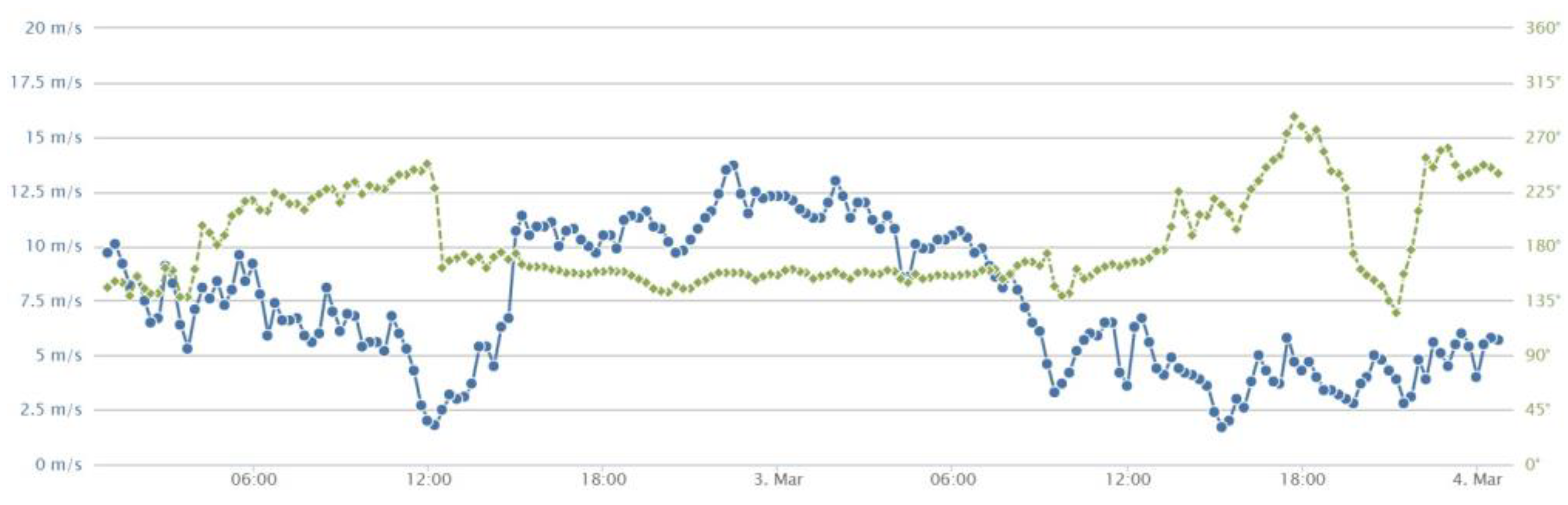
A similar synoptic condition caused the 24 November storm, however, with a weaker depression in the middle atmosphere. Again, the strongest winds blew from the south-eastern direction over the southern Apulia coast, with an intensity of 18-20 m/s (Table 2). In this case, the fetch was of about 800 km, while the duration of these conditions of about 12 h. Both the 22 December 2019 and the 2 March 2020 storms were caused by two middle atmosphere lows coming from the north-eastern direction with respect to the Italian peninsula [11]. This difference caused a different impact over the study area, with more variability of the wind speed and direction. In the case of December 2019, the prevailing direction was from the western direction over the southern Apulia coast, with a shorter fetch because of the geographic shape of the Gulf of Taranto (Figure 1). The BOLAM model shows a wind of about 14-16 m/s at 10 m over the sea, associated to a duration of 24 h and a fetch of about 400 km. In the case of March 2020, the strongest wind blew from the South, with a lower intensity of about 12-14 m/s, a duration of 12 h and a fetch of about 600 km. The calculated characteristic wave height for the storms occurred between the 24 November 2019 and the 2 March 2020 ranges from 3.4 to 4.9 m (Table 2), values lower than that of the maximum significant wave for a 50 year return period (Section 2).
Searching for the main cause of the massive displacement phenomenon occurred during the third interval time of Table 4, complementary items came from the stretches of coast that are surveyed with on-site geological observations and measures (Section 1). By surveys made after storm Detlef, 6 and 11 displaced boulders were found at Torre Suda (SUi, second displacement, SUj, SUk, SUl, SUm, SUn) and Sant'Isidoro (SIc, SIf, SIg, and 8 additional boulders that are not detected by remote sensing imagery analysis because their small size or short displacement), respectively [19,20,21] (Figure 1 for sites location). It must be noted that after storm Vaia, only one case of boulder displacement at Torre Suda site were detected (SUi, first displacement, see Figure A6a,b in Appendix A), while no displacements were found at Sant'Isidoro site.
The strong power of storm Detlef on the eastern coast of the Gulf of Taranto was also shown by the caused damage [20]. By using the Storm Power Index (SPI) introduced by Dolan and Davis (1992) [90], the intensity of the storms reported in Table 2 can be calculated. SPI is defined as the "storm’s duration times the square of maximum significant wave height" [90]. A number of studies have shown a strong correlation between SPI and the wave impact on the coasts (see e.g. [91,92,93]). Considering that H0 is nearly equivalent to the significant wave height [62,63], the storm intensities can be assessed as reported in Figure 10.
Considering the obtained values of SPI, the quite different ability of the two most severe storms to determine morphodynamic signatures in the study area is surprising. It can be guessed that the interplay between wind speed, and length and duration in time of the fetch involved, can determine a sort of threshold-like behavior between storms that do not cause massive changes (including Vaia) and the most intense one (Detlef). Moreover, by the timely distribution of the boulder displacements (Table 4), it is inferable that the storm of 22 December 2019 may have caused the change of position of some boulders. On the other hand, the 3 December 2020 storm can be considered as the most probable cause for the two displacements occurred during the interval 4. Anyway, advanced hydrodynamic modeling based on non-linear equations to also consider the TD (Tables A2, A4, A6, A8, A9, A10), could better shed light on this physical process [94,95,96].
5.3. Nearshore Wind Conditions and Wave Energy
The nearshore wind conditions during the storms of the interval 3 (Table 4), can be inferred from 2 out 3 of the wind gauge stations placed along the eastern coast of the Gulf of Taranto (Figure 1). Unfortunately, Gallipoli station was not operational during the 2019-2020 CW season (Section 3.2). The data carried out from the datasets of Santa Maria di Leuca and Porto Cesario stations are reported in Appendix B. They confirm the stronger wind conditions occurred during storm Detlef in comparison with the ones occurred during the other storms of the 2019-2020 CW season. The 12-13 November 2019, the wind speed 30 min averages measured at Santa Maria di Leuca station ranged between 15 and 18 m/s for about 24 hours, with a peak value of 24 m/s. Wind speed and duration during other storms were lower (Table B1). The measurements of the Porto Cesareo station confirm the above. The wind speed was around 20 m/s for almost the first half of November 13, while only during December 22 did it exceed 15 m/s for about 4 hours (Figure B1, B2, B3, and B4).
Usually, wind speed is significantly higher over the sea than land while wind direction is affected by more or less apparent changes in crossing the coastline. Land station measurements of wind speed can be halved in comparison with offshore values [97,98]. However, it must be noted that the Santa Maria di Leuca station has an elevation of 26 m a.s.l. and is placed about 100 m inland, while the Porto Cesareo station has an elevation of 12 m a.s.l. and is placed few tens of m inland. Since the two stations are close to the coastline, the anemometric values reported above can be considered as indicative for the nearshore conditions. The consistency with the wind speed values extracted from the GLOBO-BOLAM-MOLOCH model cascade (Section 4.3, Table 2) confirms the above.
The minimum flow velocities required to set in motion the boulders can be carefully used to assess the nearshore wave energy (Section 3.2). Regarding the study case, for the biggest boulders displaced during the 2019-2020 CW season, V ranges from 2.7 to 8.1 m/s (Table 3). Exceptional coastal storms should produce flow velocity at shore below 5 m/s [74,99]. Apparently, the displacement of some boulders (e.g., ROn, SGe) required an unusual amount of energy for flows produced by wind waves. Values of V up to 14 m/s were calculated to explain boulder displacements due to inundation events driven by typhoons in the Asia-Pacific region [74,79,100,101,102]. Instead, for the Mediterranean region, V values up to 12 m/s are reported in literature to displace SA or SB boulders [1,56]. The results of this study therefore appear to be placed in a coherent framework. However, for the use of the data in coastal hazard assessment, an improvement of the method is suggested below.
Equations (4), (5), (6), (7), (8), and (9), could provide some unreliable minimum flow velocities to set in motion the boulders due to different causes [50,76]. The first concerns the values to be attributed to the coefficients CD and CL. The drag coefficient can be affected by environmental factors and actually ranges from 1.2 to 5.0 [70,76]. On the other hand, as established by calculation and numerical simulations [78,103], the lift coefficient can be about an order of magnitude greater than the commonly used value (that is 0.178, see Section 3.2). Such an issue needs to be adequately faced as the research continues. Another set of problems concerns the real shape of the boulders and the lengths of the axes. The boulders are usually complex solids, while using the measured lengths in the equations (see Section 3 for the method; Tables A1, A3, A5, and A7 for the values), they are implicitly considered as rectangular cuboid. Consequently, the flow velocity could be overestimated because the difference between theoretical and actual size. To overcome such an issue a new approach that consider the real dimensional features of the displaced boulders, obtained by modern geophysical survey techniques, has been recently proposed [50].
Funding
This research received no external funding.
Data Availability Statement
Data supporting reported results can be found at the following links: https://protezionecivile.puglia.it/annali-e-dati-idrologici-elaborati (accessed on 10/09/2023), for the Hydrological Annals; http://www.isac.cnr.it/dinamica/projects/forecasts/index.html (accessed on 10/09/2023), for wind and wave data; http://93.51.158.171/web/simop/home (accessed on 10/09/2023), for wind data.
Acknowledgments
The author thanks: Paolo Martano for the suggestions on the description of the marine weather conditions; Luca Marzo, Luca Orlanducci, and Anna Lisa Signore for the assistance during the geomorphological surveys. The elaboration of remote sensing images (Figures 2–9) was made in the free open-source Inkscape editor.
Conflicts of Interest
The author declares no conflict of interest.
Appendix A
Data of the detected displaced boulders carried out from remote sensing resources (see Sections 3, 4), together with some features selected by field geological investigation, are reported below (Tables A1, A2, A3, A4, A5, A6, A7, and A8). Geographical coordinates and TD were taken from the September 2021 Google Earth image. Figure A1 shows the socket leaved on the parent rock by the SCa boulder (Section 4.1). The socket has been ephemeral, so that a few years after its formation it is almost indistinguishable from its rock parent (cf. Figure A1c and Figure A1b).
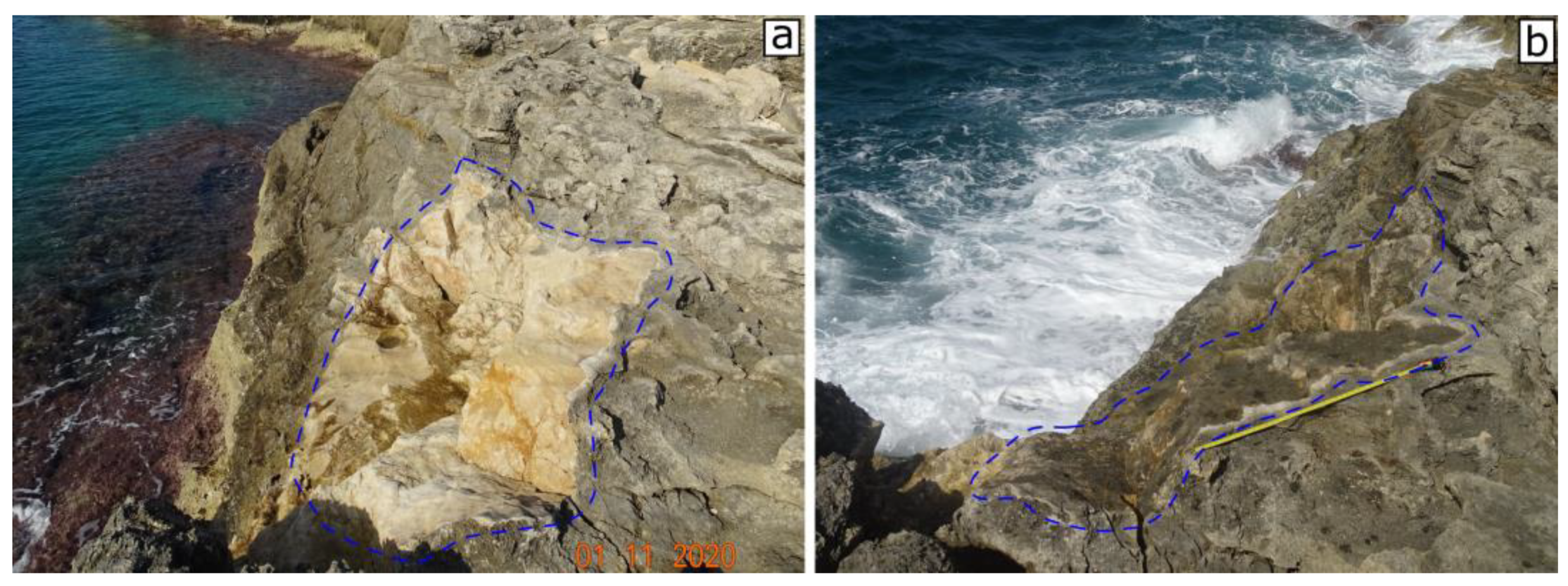
Figure A1.
Santa Caterina site; the socket leaved by the SCa boulder; (a) after about 1 year from the detachment (the image was taken the 1 November 2020), the rock surface is fresh and not weathered; (b) after about 4 years from the detachment (the image was taken the 22 September 2023, 1 m-long tape measure for scale), the rock surface is almost not distinguishable from the parent rock (cf. Figure 2d,e).
The post-transport position of SCa in unknown (Table A1). It was not recognized either from satellite images or in the field and probably SCa fell into the sea after detaching from its initial position.

Table A1.
Initial (pre-displacement) and final (post-displacement) geographical coordinates of the storm-displaced boulders at Santa Caterina coast; ind., indeterminable. A.I., annual interval in which the displacement occurred (cf. Table 4).
Table A1.
Initial (pre-displacement) and final (post-displacement) geographical coordinates of the storm-displaced boulders at Santa Caterina coast; ind., indeterminable. A.I., annual interval in which the displacement occurred (cf. Table 4).
| Initial position | Final position | ||||
| ID | latitude | longitude | latitude | longitude | A.I. |
| SCa | 40°08'17.09"N | 17°59'19.21"E | ind. | ind. | 3 |
| SCb | 40°08'18.36"N | 17°59'18.47"E | 40°08'19.03"N | 17°59'18.85"E | 3 |
Differently from the socket of SCa, due to the different distance to the coastal cliff (Table A2), the surface of the SCb boulder is still fresh and unaltered (Figure A2). Moreover, since SCb lies on a shrub vegetation area, it is easily recognizable in remote sensing images (cf. Figure 2d,e).
Figure A2.
Santa Caterina site; the SCb boulder after the displacement occurred between July 2019 and September 2020 (the image was taken the 22 September 2023, 1 m-long tape measure for scale). The whitish surface of SCb is uncovered by lichen, therefore still easily detectable in the field as well as by remote sensing images (see Section 4.1).
Table A2.
Main features of the storm-displaced boulders at Santa Caterina coast; major and middle axes measured on remote sensing imagery ar, br (in m); dimensions of the axes taken in the field af, bf, cf (in m); inclination on the ground I; initial distances from the coastline xi, final distances from the coastline xf (in m). TD, Transport Distance; Li, Lithology: C, Calcarenite, L, Limestone; Sh, Shape: O, Oblate (b/a > 0.6, c/b < 0.6), E, Equant (b/a > 0.6, c/b > 0.6), B, Bladed(b/a < 0.6, c/b < 0.6), P, Prolate (b/a < 0.6, c/b > 0.6); FI, Flatness Index; PTS, Pre Transport Setting: JB, Joint-Bounded, SA, Sub-Aerial, SB, Submerged, CE, Cliff-edge; MT, Movement Type: ST, saltation, SL, sliding, OV, overturning; ind., indeterminable.
| ID | ar | br | af | bf | cf | I | xi | xf | TD | Li | Sh | FI | PTS | MT |
| SCa | 3.3 | 1.2 | - | - | - | - | 0.8 | ind. | - | L | - | - | CE | - |
| SCb | 1.8 | 1.5 | 1.8 | 1.6 | 0.7 | 5° | 18.8 | 21.6 | 15.4 | L | O | 2.5 | SA | OV |
Table A3.
Initial (pre-displacement) and final (post-displacement) geographical coordinates of the storm-displaced boulders at Pilella coast; see caption of Table A1 for symbols.
Table A3.
Initial (pre-displacement) and final (post-displacement) geographical coordinates of the storm-displaced boulders at Pilella coast; see caption of Table A1 for symbols.
| Initial position | Final position | ||||
| ID | latitude | longitude | latitude | longitude | A.I. |
| PILa | 39°55'22.66"N | 18°03'35.76"E | 39°55'22.72"N | 18°03'35.80"E | 3 |
| PILb | 39°55'22.60"N | 18°03'35.42"E | 39°55'22.68"N | 18°03'35.51"E | 3 |
| PILc | 39°55'22.27"N | 18°03'34.62"E | 39°55'22.35"N | 18°03'34.66"E | 2 or 3 |
| PILd | 39°55'22.24"N | 18°03'34.49"E | 39°55'22.33"N | 18°03'34.50"E | 3 |
| PILe | ind. | ind. | 39°55'23.54"N | 18°03'32.43"E | 3 |
| PILf | 39°55'23.83"N | 18°03'31.60"E | 39°55'23.88"N | 18°03'31.63"E | 3 |
| PILg | 39°55'23.97"N | 18°03'31.61"E | 39°55'24.11"N | 18°03'31.72"E | 3 |
| PILh | ind. | ind. | 39°55'24.08"N | 18°03'30.58"E | 3 |
| PILi | 39°55'24.39"N | 18°03'31.08"E | 39°55'24.49"N | 18°03'31.12"E | 3 |
| PILj | 39°55'25.09"N | 18°03'27.70"E | 39°55'25.10"N | 18°03'27.78"E | 3 |
| PILk | 39°55'25.38"N | 18°03'27.86"E | ind. | ind. | 3 |
| PILl | 39°55'26.41"N | 18°03'27.20"E | 39°55'26.49"N | 18°03'27.26"E | 3 |
| PILm | 39°55'26.86"N | 18°03'26.56"E | 39°55'26.96"N | 18°03'26.64"E | 3 |
| PILn | 39°55'27.29"N | 18°03'26.47"E | 39°55'27.32"N | 18°03'26.54"E | 3 |
Several displaced boulders show a high value of I. As an example, the PILn boulder (Figure A3) is inclined of about 55° with respect to the ground (Table A4). Such an arrangement can cause the underestimation of the horizontal dimensions of the boulders from remote sensing imagery (Section 4).
Figure A3.
Pilella site; the PILn boulder lies on a smaller boulder and form an angle of about 55° with respect to the ground. Note the difference in length between br and bf (see the caption of Table A2 for symbols).
Figure A3.
Pilella site; the PILn boulder lies on a smaller boulder and form an angle of about 55° with respect to the ground. Note the difference in length between br and bf (see the caption of Table A2 for symbols).
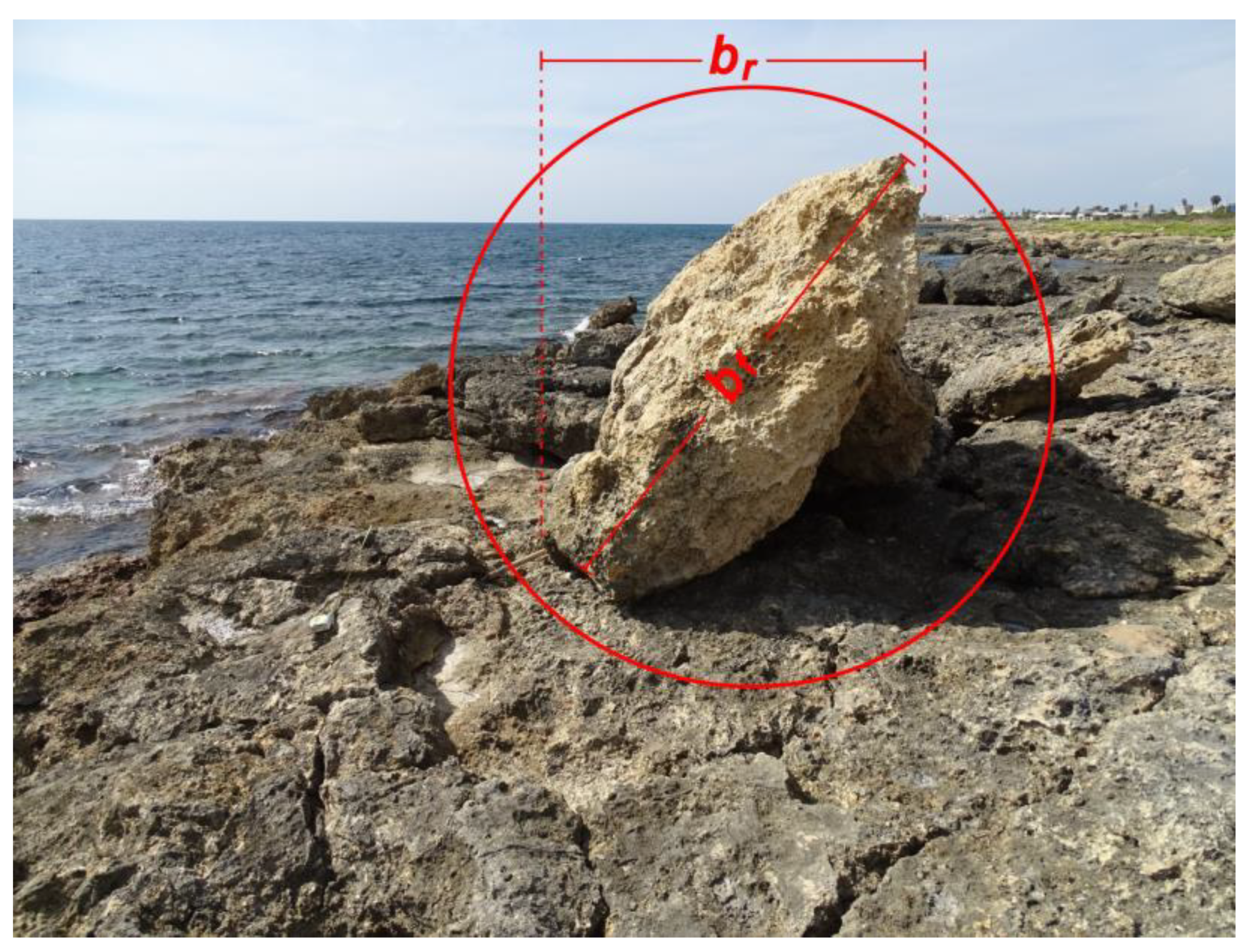
Table A4.
Main features of the storm-displaced boulders at Pilella coast; see caption of Table A2 for symbols.
Table A4.
Main features of the storm-displaced boulders at Pilella coast; see caption of Table A2 for symbols.
| ID | ar | br | af | bf | cf | I | xi | xf | TD | Li | Sh | FI | PTS | MT |
| PILa | 1.6 | 0.9 | 1.6 | 1.0 | 0.5 | 0-5° | 10.8 | 12.4 | 3.6 | C | O | 2.6 | SA | OV |
| PILb | 2.0 | 1.0 | 1.8 | 1.0 | 0.4 | 0-5° | 9.4 | 10.5 | 4.1 | C | B | 3.5 | SA | OV |
| PILc | 1.5 | 1.0 | 1.5 | 0.9 | 0.4 | ~20° | 12.4 | 14.7 | 2.5 | C | B | 3 | SA | OV |
| PILd | 2.0 | 1.2 | 1.9 | 1.0 | 0.6 | 0-5° | 13.6 | 15.6 | 2.6 | C | B | 2.4 | SA | OV |
| PILe | 2.3 | 1.6 | 2.5 | 1.5 | 0.3 | ~15° | ind. | 13.2 | - | C | O | 6.7 | SA,SB | ST,OV |
| PILf | 2.2 | 1.5 | 2.4 | 1.2 | 0.5 | ~60° | 10.9 | 12.5 | 1.5 | C | B | 3.6 | SA | SL |
| PILg | 1.7 | 1.4 | 1.5 | 1.3 | 0.6 | ~10° | 10.6 | 15.5 | 4.8 | C | O | 2.3 | SA | OV |
| PILh | 2.2 | 1.0 | 1.9 | 1.0 | 0.5 | 5° | ind. | 3.9 | - | L | B | 2.9 | SA,SB | ind. |
| PILi | 1.9 | 1.1 | 2.2 | 1.1 | 0.4 | 5° | 18.8 | 20.4 | 2.6 | C | B | 4.1 | SA | ST |
| PILj | 3.1 | 1.9 | 3.0 | 1.8 | 0.6 | 5° | 0.7 | 1.9 | 1.6 | C | O | 4 | SB | SL |
| PILk | 2.0 | 1.4 | - | - | - | - | 6.9 | ind. | - | - | - | - | SA | - |
| PILl | 2.0 | 1.1 | 2.1 | 1.1 | 0.8 | 0-5° | 7.0 | 8.9 | 3.3 | L | P | 2 | SA | OV |
| PILm | 2.1 | 1.1 | 2.0 | 1.0 | 0.4 | 0-5° | 1.1 | 3.7 | 3.2 | C | B | 3.7 | SA | OV |
| PILn | 2.2 | 1.2 | 2.1 | 1.8 | 0.4 | ~55° | 4.4 | 6.2 | 1.9 | C | O | 4.9 | SA | OV |
Table A5.
Initial (pre-displacement) and final (post-displacement) geographical coordinates of the storm-displaced boulders at Posto Rosso coast; see caption of Table A1 for symbols.
Table A5.
Initial (pre-displacement) and final (post-displacement) geographical coordinates of the storm-displaced boulders at Posto Rosso coast; see caption of Table A1 for symbols.
| Initial position | Final position | ||||
| ID | latitude | longitude | latitude | longitude | A.I. |
| ROa | 30°54'45.53"N | 18°04'20.88"E | 30°54'47.70"N | 18°04'20.99"E | 3 |
| ROb | 30°54'46.19"N | 18°04'20.51"E | 30°54'46.21"N | 18°04'20.55"E | 3 |
| ROc | 30°54'46.87"N | 18°04'20.58"E | 30°54'46.90"N | 18°04'20.69"E | 3 |
| ROd | 30°54'47.88"N | 18°04'18.76"E | 30°54'48.03"N | 18°04'18.79"E | 3 |
| ROe | ind. | ind. | 30°54'48.30"N | 18°04'17.88"E | 3 |
| ROf | 30°54'48.40"N | 18°04'17.90"E | 30°54'48.45"N | 18°04'17.96"E | 3 |
| ROg | ind. | ind. | 30°54'48.39"N | 18°04'17.57"E | 3 |
| ROh | ind. | ind. | 30°54'48.43"N | 18°04'17.54"E | 3 |
| ROi | 30°54'48.38"N | 18°04'17.34"E | 30°54'48.44"N | 18°04'17.36"E | 3 |
| ROj | 30°54'48.40"N | 18°04'17.44"E | 30°54'48.51"N | 18°04'17.47"E | 3 |
| ROk | 30°54'48.45"N | 18°04'17.59"E | 30°54'48.52"N | 18°04'17.37"E | 3 |
| ROl | ind. | ind. | 30°54'48.79"N | 18°04'17.15"E | 4 |
| ROm | 30°54'49.29"N | 18°04'16.85"E | 30°54'49.40"N | 18°04'16.95"E | 3 |
| ROn | 30°54'49.02"N | 18°04'15.97"E | 30°54'48.48"N | 18°04'16.41"E | 3 |
| ROo | ind. | ind. | 30°54'49.68"N | 18°04'16.38"E | 2 or 3 |
| ROp | ind. | ind. | 30°54'49.71"N | 18°04'16.43"E | 2 or 3 |
Figure A4.
Posto Rosso site; (a) the overturned ROa boulder and (in the foreground) its socket (1 m-long tape measure for scale); (b) the geomorphological arrangement of ROl boulder, that was displaced during the 2019–2020 CW season (see Section 4.1); (c) the socket of the ROn boulder; (d) the ROn boulder was detached from its initial position and displaced of about 17 m inland.
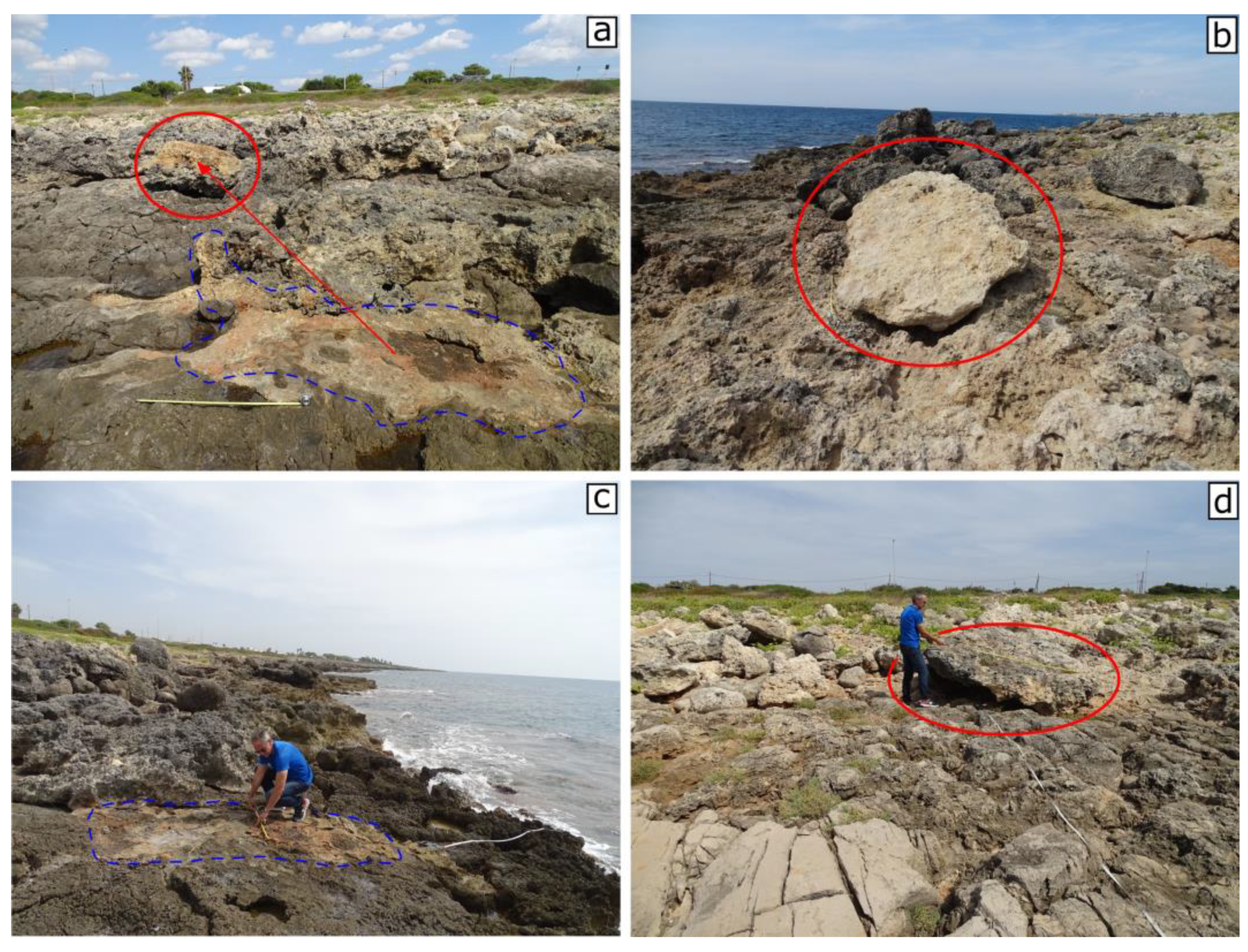
Many coarse boulders have been detected at Posto Rosso site (Section 4.1, Table A6). The ROa boulder was detached and overturned (Figure A4a). The boulder ROl also appears to have been overturned (Figure A4b). The ROn boulder, despite its large size was transported for 17 m due to the water flow (Figure A4c,d).
Table A6.
Main features of the storm-displaced boulders at Posto Rosso coast; see caption of Table A2 for symbols.
Table A6.
Main features of the storm-displaced boulders at Posto Rosso coast; see caption of Table A2 for symbols.
| ID | ar | br | af | bf | cf | I | xi | xf | TD | Li | Sh | FI | PTS | MT |
| ROa | 2.7 | 1.4 | 2.7 | 1.3 | 0.8 | 0-5° | 12.3 | 18.5 | 5.8 | C | P | 2.5 | SA | OV |
| ROb | 2.8 | 1.3 | 2.9 | 1.4 | 0.6 | 0-5° | 5.7 | 6.7 | 1.9 | C | B | 3.6 | SA | SL |
| ROc | 1.6 | 1.3 | 1.7 | 1.4 | 0.5 | 0-5° | 15.9 | 18.2 | 2.5 | C | O | 3.1 | SA | ST |
| ROd | 2.5 | 1.9 | 2.4 | 1.5 | 0.7 | ~20° | 10.4 | 14.7 | 4.5 | C | O | 2.8 | SA | OV |
| ROe | 2.1 | 1.6 | 2.3 | 1.6 | 0.5 | 0-5° | ind. | 11.2 | - | C | O | 3.9 | SA,SB | ind. |
| ROf | 1.8 | 1.4 | 1.7 | 1.4 | 0.7 | 0-5° | 13.6 | 15.8 | 2.1 | C | O | 2.2 | SA | ST |
| ROg | 1.5 | 0.9 | 1.3 | 0.9 | 0.4 | ~25° | ind. | 14.6 | - | C | B | 2.7 | SA,SB | ST |
| ROh | 1.6 | 0.9 | 1.7 | 0.9 | 0.7 | 0-5° | ind. | 14.4 | - | C | P | 1.8 | SA,SB | ST |
| ROi | 2.8 | 1.3 | 2.7 | 1.4 | 0.7 | ~10° | 11.1 | 12.6 | 1.9 | C | B | 2.9 | SA | ST |
| ROj | 2.6 | 1.5 | 2.4 | 1.7 | 0.8 | ~20° | 14.4 | 16.7 | 3.1 | C | B | 2.6 | SA | OV |
| ROk | 1.7 | 1.2 | 1.7 | 1.3 | 0.7 | ~15° | 14.2 | 16.1 | 2.1 | C | O | 2.1 | SA | OV |
| ROl | 1.8 | 1.3 | 1.9 | 1.2 | 0.3 | ~20° | ind. | 9.3 | - | C | O | 5.2 | SA,SB | OV |
| ROm | 1.5 | 0.8 | 1.4 | 0.8 | 0.5 | 0-5° | 20.3 | 25.2 | 4.8 | C | P | 2.2 | SA | ST |
| ROn | 3.1 | 1.8 | 2.8 | 2.1 | 0.5 | ~20° | 4.2 | 20.7 | 17.1 | C | O | 4.9 | SA | ST |
| ROo | 1.3 | 0.9 | 1.4 | 0.9 | 0.5 | ~10° | ind. | 25.3 | - | C | B | 2.3 | SA,SB | ST,OV |
| ROp | 1.5 | 0.8 | 1.7 | 1.1 | 0.5 | ~25° | ind. | 26.4 | - | C | O | 2.8 | SA,SB | ST,OV |
Table A7.
Initial (pre-displacement) and final (post-displacement) geographical coordinates of the storm-displaced boulders at Torre San Giovanni coast; see caption of Table A1 for symbols.
Table A7.
Initial (pre-displacement) and final (post-displacement) geographical coordinates of the storm-displaced boulders at Torre San Giovanni coast; see caption of Table A1 for symbols.
| Initial position | Final position | ||||
| ID | latitude | longitude | latitude | longitude | A.I. |
| SGa | ind. | ind. | 39°54'03.86"N | 18°05'09.25"E | 3 |
| SGb | ind. | ind. | 39°54'03.99"N | 18°05'09.47"E | 3 |
| SGc | ind. | ind. | 39°54'04.46"N | 18°05'09.50"E | 3 |
| SGd | 39°54'04.18"N | 18°05'09.34"E | 39°54'04.49"N | 18°05'09.38"E | 3 |
| SGe | 39°54'04.52"N | 18°05'08.72"E | 39°54'04.73"N | 18°05'08.76"E | 3 |
| SGf | 39°54'05.57"N | 18°05'08.45"E | 39°54'05.61"N | 18°05'08.53"E | 3 |
Several of the displaced boulders are rather flatness (e.g., PILe and SGd; see Table A4 and Table A8, respectively). The flat SGd boulder (FI = 6, Figure A5) was transported for almost 10 m from an initial position more than 20 m away from the coastline.
Figure A5.
Torre San Giovanni site; SGc (in the foreground) and SGd boulders. As a result of the water flow transport, they have formed two imbricated clusters together with other small boulders.
Figure A5.
Torre San Giovanni site; SGc (in the foreground) and SGd boulders. As a result of the water flow transport, they have formed two imbricated clusters together with other small boulders.
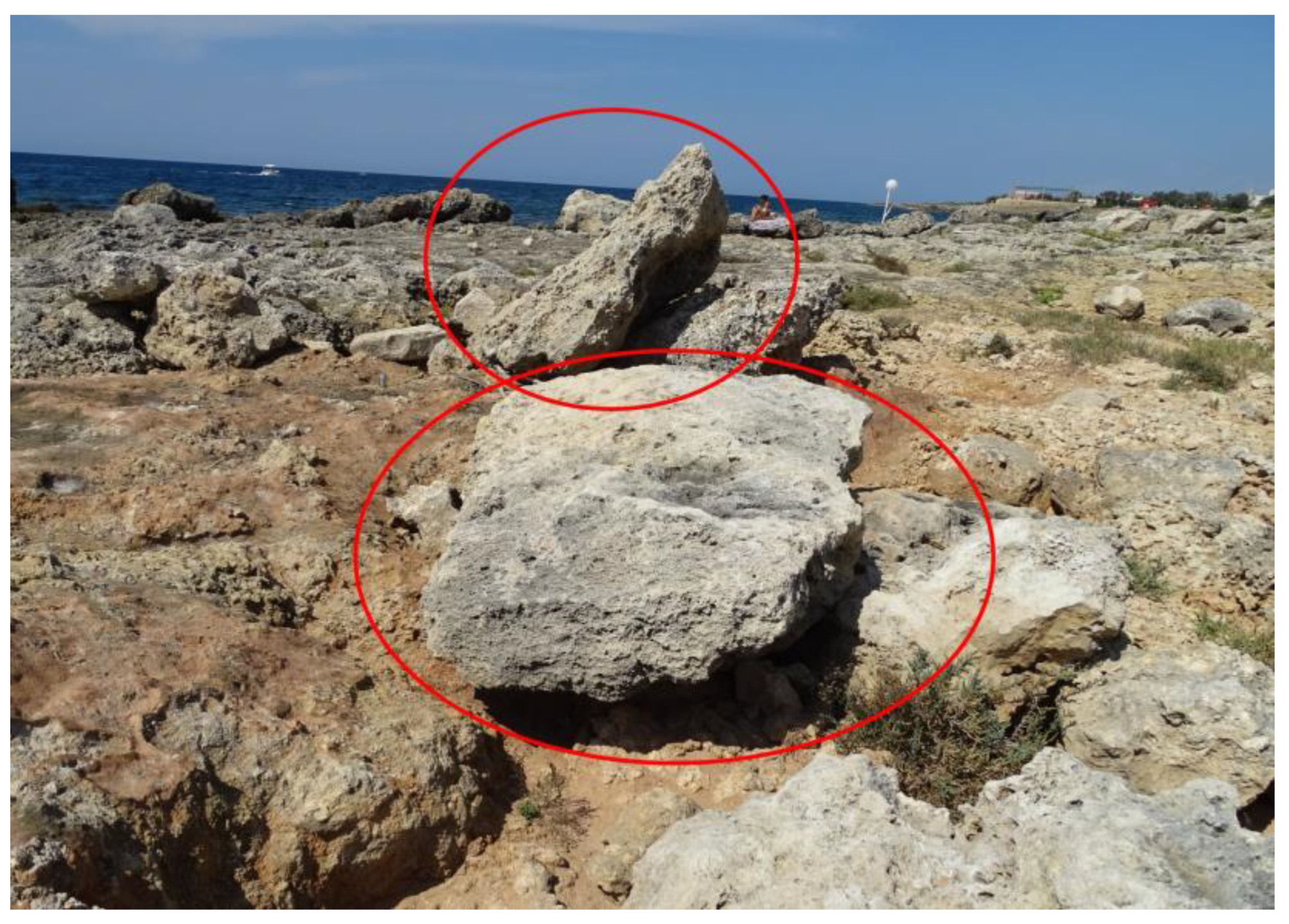
Table A8.
Main features of the storm-displaced boulders at Torre San Giovanni coast; see caption of Table A2 for symbols.
Table A8.
Main features of the storm-displaced boulders at Torre San Giovanni coast; see caption of Table A2 for symbols.
| ID | ar | br | af | bf | cf | I | xi | xf | TD | Li | Sh | FI | PTS | MT |
| SGa | 1.5 | 0.9 | 1.4 | 1.1 | 0.4 | 0-5° | ind. | 14.9 | - | C | O | 3.1 | SA,SB | ST,OV |
| SGb | 1.8 | 1.1 | 1.8 | 1.0 | 0.3 | 0-5° | ind. | 22.3 | - | C | B | 4.7 | SA,SB | ST,OV |
| SGc | 1.9 | 1.1 | 1.8 | 1.2 | 0.3 | 0-5° | ind. | 31.4 | - | C | O | 5 | SA,SB | ST,OV |
| SGd | 2.1 | 0.9 | 2.3 | 1.3 | 0.3 | ~45° | 22.8 | 28.6 | 9.5 | C | B | 6 | SA | ST |
| SGe | 2.4 | 1.7 | 2.2 | 1.7 | 0.7 | 0-5° | 13.8 | 18.2 | 6.5 | C | O | 2.8 | SA | ST |
| SGf | 1.6 | 0.8 | 1.5 | 1.2 | 0.6 | ~30° | 10.4 | 11.7 | 2.4 | C | O | 2.2 | SA | OV |
When both the initial and final positions of the detected boulders were established, the transport distance was calculated (Section 4.1, 4.2). In the Table A9 and Table A10 the lists of these boulders are reported.
Table A9.
Displaced boulders detected in this study for which TD was calculated and whose position changes between July 2019 and June 2020.
Table A9.
Displaced boulders detected in this study for which TD was calculated and whose position changes between July 2019 and June 2020.
| Site | Boulder ID1 |
|---|---|
| Santa Caterina | SCa |
| Pilella | PILa, PILb, PILc, PILd, PILf, PILg, PILi, PILj, PILl, PILm, PILn |
| Posto Rosso | ROa, ROb, ROc, ROd, ROf, ROi, ROj, ROk, ROm, ROn |
| Torre San Giovanni | SGd, SGe, SGf |
1 for geographical coordinates, transport distance, dimensions of the axes, pre- and post-displacement distances from the coastline, lithology, shape, flatness index, pre-displacement setting, and movement type, see Table A1, Table A2, Table A3, Table A4, Table A5, Table A6 and Table A7, and A8.
Table A10.
Displaced boulders detected by [11] whose position results changed between July 2019 and June 2020 and for which TD was calculated.
Table A10.
Displaced boulders detected by [11] whose position results changed between July 2019 and June 2020 and for which TD was calculated.
| Site | Boulder ID1 |
|---|---|
| Punta Prosciutto | PRa, PRb, PRc, PRd, PRe, PRf, PRi, PRj, PRk, PRl, PRm, PRq, PRr |
| Sant’Isidoro | SIf, SIg |
| Punta Pizzo | PIa, PIb, PIc, PId, PIe, PIg, PIh, PIj, PIn, PIp, PIr |
| Mancaversa | MAa, MAb, MAc, MAf, MAg, MAh, MAi, MAj, MAk, MAl, MAm |
| Torre Suda | SUa, SUe, SUf, SUh, SUi, SUn |
| Capilungo | CAa, CAb, CAc, CAd, CAe, CAf |
| Ciardo | CIa, CIb, CIc, CId |
1 for geographical coordinates, transport distance, dimensions of the axes, pre- and post-displacement distances from the coastline, lithology, shape, flatness index, pre-displacement setting, and movement type, see Appendix A in Delle Rose et al. (2021) [11].
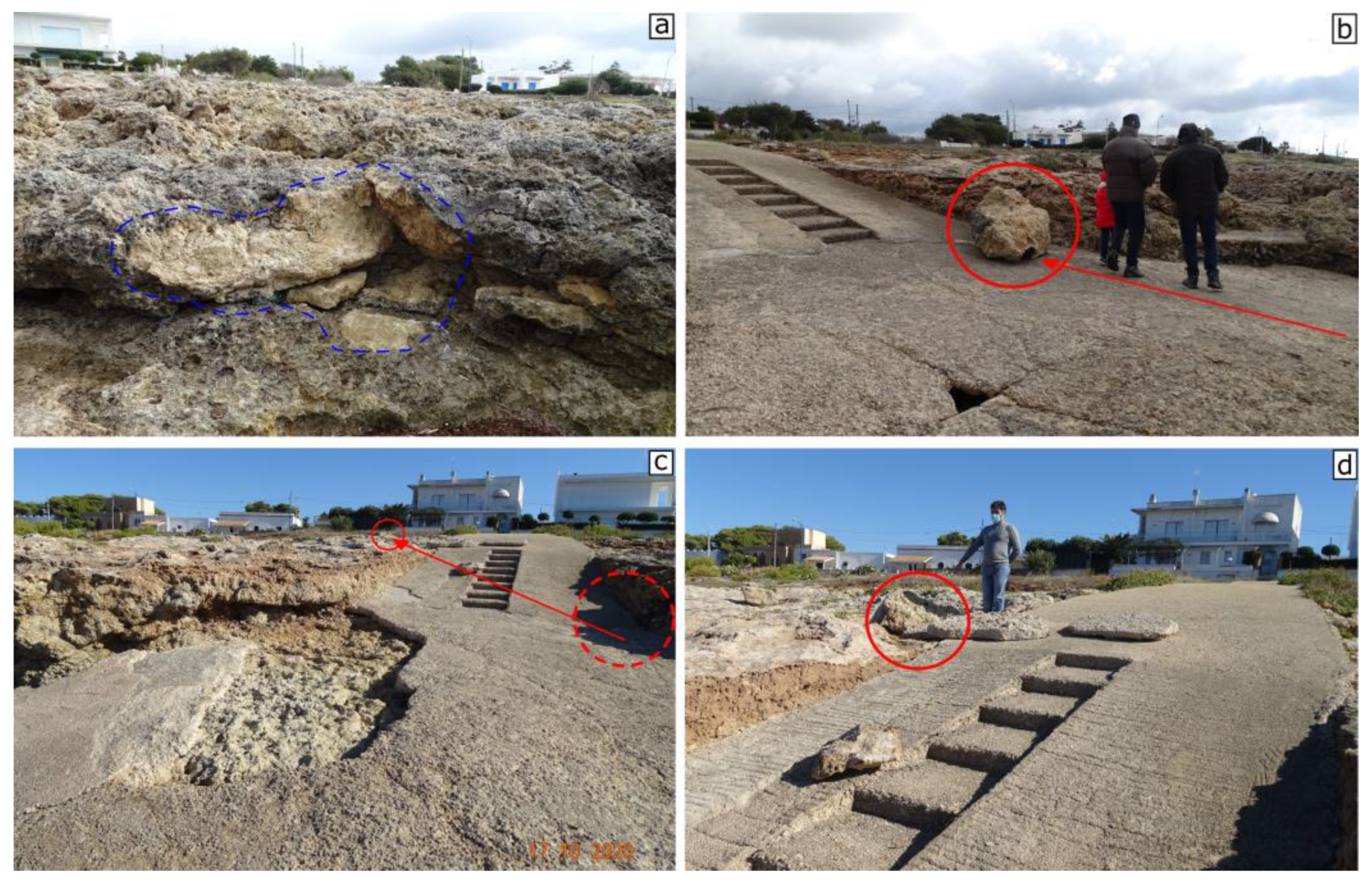
As above reported (section 4), two boulders underwent two displacements during the 2017-2021. In the case of the SUi boulder (Section 4.2), this singular mobility can be due to the presence of a slipway ramp that channel the water flows (Figure A6).
Figure A6.
Torre Suda site; (a) the socket of the SUi boulder (image taken the 23 February 2019); (b) the SUi boulder lying on a slipway ramp after the first movement (image taken the 23 February 2019); (c); (d) the SUi boulder displaced out of the ramp due to the second movement (images taken the 17 October 2020).
With the aim to best calculate the flow velocities of Table 3, the geomorphological setting of the boulders detected by [11] has been revised. Thus, detailed observations have been made on the ground surface and rock joints. For the pre transport setting (PTS) of the MAa boulder (previous considered as joint-bounded), the result of the on-site survey (no fresh surface delimited MAa) suggested to consider it as subaerial (SA). Instead, for the other boulders of Table 3, it was confirmed the previously established PTS.
Figure A7.
Mancaversa site; the MAa boulder lying about 4.5 m from its initial position (in the foreground); rock joints are indicated by green arrows (see text).
Figure A7.
Mancaversa site; the MAa boulder lying about 4.5 m from its initial position (in the foreground); rock joints are indicated by green arrows (see text).

Appendix B
2019-2020 Data carried out from the datasets of Santa Maria di Leuca (Table B1) and Porto Cesario stations (Figures B1, B2, B3, and B4) are reported below (see Section 5.3).
Table B1.
Wind speed daily average (Ua), wind speed daily maximum (Um), and 30 min averages wind speed (U30) and direction (D) at four selected hours. Data recorded by the Santa Maria di Leuca wind gauge (data extracted from [66,67]).
| 00:00 | 06:00 | 12:00 | 18:00 | |||||||
| Storm | Ua | Um | U30 | D | U30 | D | U30 | D | U30 | D |
| 12/11/20191 | 8.5 | 24.0 | 9.8 | 106° | 18.1 | 107° | 13.4 | 145° | 11.7 | 164° |
| 13/11/20191 | 6.0 | 19.8 | 15.4 | 169° | 12.7 | 167° | 12.1 | 173° | 4.3 | 172° |
| 24/11/2019 | 5.5 | 19.3 | 4.9 | 145° | 7.4 | 129° | 14.5 | 107° | 16.3 | 112° |
| 22/12/2019 | 4.9 | 18.1 | 8.2 | 191° | 9.4 | 179° | 14.0 | 222° | 7.8 | 259° |
| 02/03/2020 | 3.7 | 12.7 | 7.4 | 153° | 3.0 | 53° | 6.1 | 139° | 8.3 | 146° |
1 Storm Detlef.
Figure B1.
Wind speed and direction (dashed line) recorded by the Porto Cesareo wind gauge during the storm Detlef; image downloaded 13 November 2023 from the site of the Apulian Meteomarine Network [69].
Figure B1.
Wind speed and direction (dashed line) recorded by the Porto Cesareo wind gauge during the storm Detlef; image downloaded 13 November 2023 from the site of the Apulian Meteomarine Network [69].
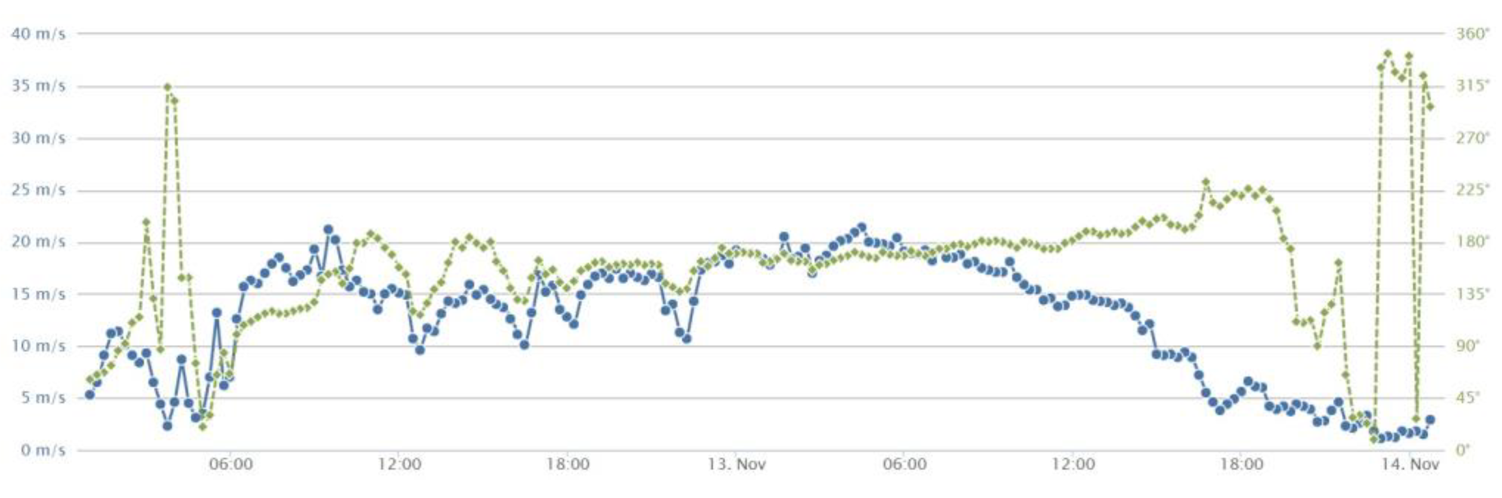
Figure B2.
Wind speed and direction (dashed line) recorded by the Porto Cesareo wind gauge during the 24 November 2019 storm; image downloaded 13 November 2023 from the site of the Apulian Meteomarine Network [69].
Figure B2.
Wind speed and direction (dashed line) recorded by the Porto Cesareo wind gauge during the 24 November 2019 storm; image downloaded 13 November 2023 from the site of the Apulian Meteomarine Network [69].
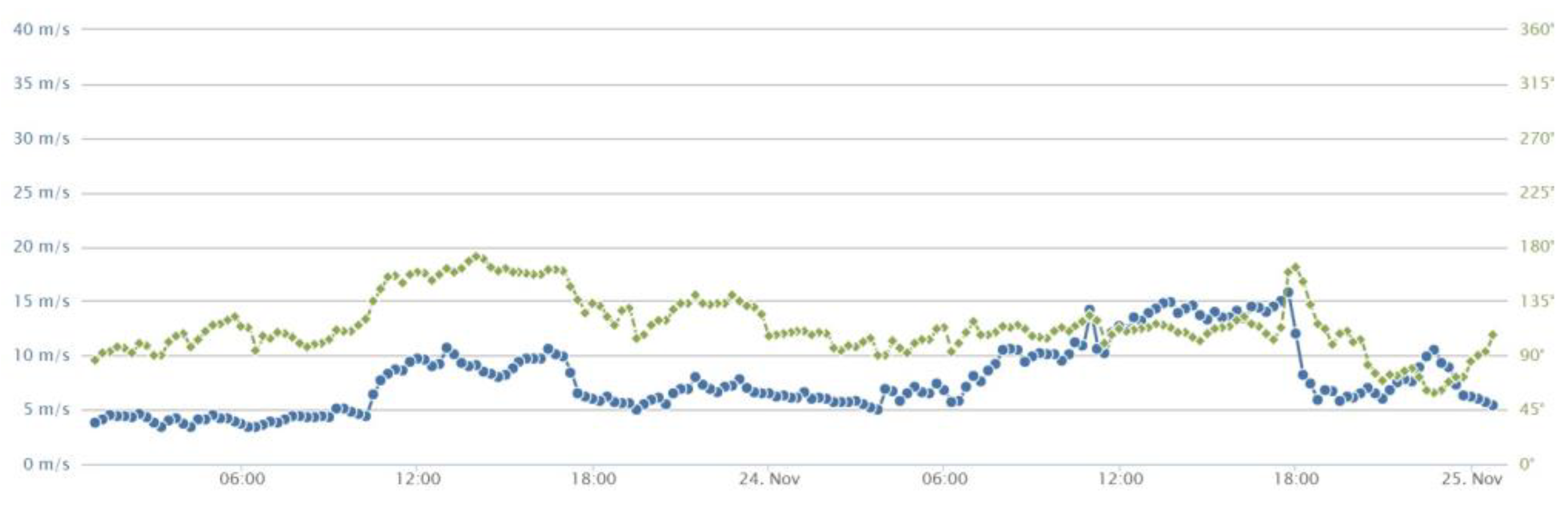
Figure B3.
Wind speed and direction (dashed line) recorded by the Porto Cesareo wind gauge during the 22 December 2019 storm; image downloaded 13 November 2023 from the site of the Apulian Meteomarine Network [69].
Figure B3.
Wind speed and direction (dashed line) recorded by the Porto Cesareo wind gauge during the 22 December 2019 storm; image downloaded 13 November 2023 from the site of the Apulian Meteomarine Network [69].
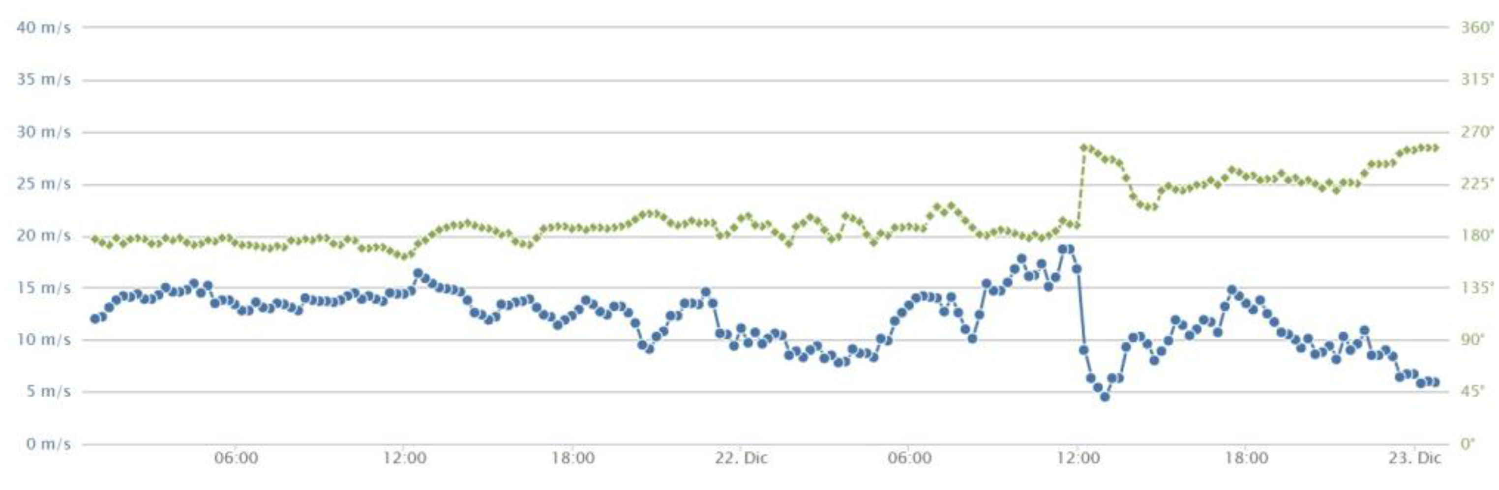
Figure B4.
Wind speed and direction (dashed line) recorded by the Porto Cesareo wind gauge during the 2 March 2020 storm; image downloaded 13 November 2023 from the site of the Apulian Meteomarine Network [69].
Figure B4.
Wind speed and direction (dashed line) recorded by the Porto Cesareo wind gauge during the 2 March 2020 storm; image downloaded 13 November 2023 from the site of the Apulian Meteomarine Network [69].
References
- Nandasena, N.A.K.; Paris, R.; Tanaka, N. Reassessment of hydrodynamic equations to initiate boulder transport by high energy events (storms, tsunamis). Mar. Geol. 2011, 281, 70–84. [Google Scholar] [CrossRef]
- Kennedy, A.B.; Cox, R.; Dias, F. Storm waves may be the source of some “tsunami” coastal boulder deposits. Geophys. Res. Lett. 2021, 48, e2020GL090775. [Google Scholar] [CrossRef]
- Delle Rose, M.; Martano, P. The Imprint of Recent Meteorological Events on Boulder Deposits along the Mediterranean Rocky Coasts. Climate 2022, 10, 94. [Google Scholar] [CrossRef]
- Collin, A.; Etienne, S.; Planes, S. High-energy events, boulder deposits and the use of very high resolution remote sensing in coral reef environments. J. Coastal Res. Special Issue 2013, 65, 690–695. [Google Scholar] [CrossRef]
- Collin, A.; Etienne, S.; Jeanson, M. Three-dimensional structure of coral reef boulders transported by stormy waves using the very high resolution WorldView-2 satellite. J. Coastal Res. Special Issue 2016, 75, 572–576. [Google Scholar] [CrossRef]
- Cox, R. Megagravel deposits on the west coast of Ireland show the impacts of severe storms. Weather 2020, 75, 72–77. [Google Scholar] [CrossRef]
- Ruban, D.A. Finding Coastal Megaclast Deposits: A Virtual Perspective. J. Mar. Sci. Eng. 2020, 8, 164. [Google Scholar] [CrossRef]
- Kennedy, A.B.; Mori, N.; Yasuda, T.; Shimozono, T.; Tomiczek, T.; Donahue, A.; Shimura, T.; Imai, Y. Extreme block and boulder transport along a cliffed coastline (Calicoan Island, Philippines) during Super Typhoon Haiyan. Mar. Geol. 2017, 383, 65–77. [Google Scholar] [CrossRef]
- Medina, F.; Mhammdi, N.; Emran, A.; Hakdaoui, S. A case of uplift and transport of a large boulder by the recent winter storms at Dahomey beach (Morocco). In Proceedings of the IX Symposium on the Iberian Atlantic Margin, Coimbra, Portugal, 4-7 September 2018; 2 pp. [Google Scholar]
- Haslett, S.; Wong, B. Reconnaissance survey of coastal boulders in the Moro Gulf (Philippines) using Google Earth imagery: Initial insights into Celebes Sea tsunami events. Bull. Geol. Soc. Malaysia 2019, 68, 37–44. [Google Scholar] [CrossRef]
- Delle Rose, M.; Martano, P.; Orlanducci, L. Coastal Boulder Dynamics Inferred from Multi-Temporal Satellite Imagery, Geological and Meteorological Investigations in Southern Apulia, Italy. Water 2021, 13, 2426. [Google Scholar] [CrossRef]
- Kennedy, D.M.; Woods, J.L.D.; Naylor, L.A.; Hansom, J.D.; Rosser, N.J. Intertidal boulder-based wave hindcasting can underestimate wave size: Evidence from Yorkshire, UK. Mar. Geol. 2019, 411, 98–106. [Google Scholar] [CrossRef]
- Hastewell, L.J.; Schaefer, M.; Bray, M.; Inkpen, R. Intertidal boulder transport: A proposed methodology adopting Radio Frequency Identification (RFID) technology to quantify storm induced boulder mobility. Earth Surf. Process. Landforms 2019, 44, 681–698. [Google Scholar] [CrossRef]
- Gomez-Pazo, A.; Perez-Alberti, A.; Trenhaile, A. Tracking clast mobility using RFID sensors on a boulder beach in Galicia, NW Spain. Geomorphology 2021, 373, 107514. [Google Scholar] [CrossRef]
- Autret, R.; Dodet, G.; Suanez, S.; Roudaut, G.; Fichaut, B. Long–term variability of supratidal coastal boulder activation in Brittany (France). Geomorphology 2018, 304, 184–200. [Google Scholar] [CrossRef]
- Hoffmeister, D.; Curdt, C; Bareth, G. Monitoring the sedimentary budget and dislocated boulders in western Greece—Results since 2008. Sedimentology 2020, 67, 1411–1430. [Google Scholar] [CrossRef]
- Morucci, S.; Picone, M.; Nardone, G.; Arena, G. Tides and waves in the central Mediterranean Sea. J. Oper. Oceanogr. 2016, 9, s10–s17. [Google Scholar] [CrossRef]
- Dentale, F.; Furcolo, P.; Pugliese Carratelli, E.; Reale, F.; Contestabile, P.; Tomasicchio, G.R. Extreme wave analysis by integrating model and wave buoy data. Water 2018, 10, 373. [Google Scholar] [CrossRef]
- Ciricugno, L.; Delle Rose, M.; Fidelibus, C.; Orlanducci, L.; Mangia, M. Sullo spostamento di massi costieri causato da onde “estreme” (costa ionica salentina). Geol. Territ. 2019, 16, 15–23. (In Italian) [Google Scholar]
- Delle Rose, M. , Fidelibus, C.; Martano, P.; Orlanducci, L. Storm-induced boulder displacements: Inferences from field surveys and hydrodynamic equations. Geosciences 2020, 10, 374. [Google Scholar] [CrossRef]
- Delle Rose, M.; Ciricugno, L.; Fidelibus, C.; Martano, P.; Marzo. L.; Orlanducci, L. Considerazioni geologiche su processi morfodinamici causati sulla costa ionica salentina da recenti tempeste. Geol. Territ. 2020, 18, 5–15. (In Italian) [Google Scholar]
- Spano, D.; Snyder, R.L.; Cesaraccio, C. Mediterranean Climates. In Phenology: An Integrative Environmental Science; Schwartz, M.D., Ed.; Springer: Dordrecht, Netherlands, 2003; pp. 139–156. [Google Scholar]
- Lionello, P.; Malanotte-Rizzoli, P.; Boscolo, R.; Alpert, P.; Artale, V.; Li, L.; Luterbacher, J.; May,W. ; Trigo, R.; Tsimplis, M.; et al. The Mediterranean Climate: An Overview of the Main Characteristics and Issues. Dev. Earth Environ. Sci. 2006, 4, 1–26. [Google Scholar]
- Zito, G.; Ruggiero, L.; Zuanni, F. Aspetti meteorologici e climatici della Puglia. In Proceedings of the First Workshop on “Clima, Ambiente e Territorio nel Mezzogiorno”, Taormina, Italy, 11–12 December 1989; CNR: Roma, Italy, 1991; pp. 43–73. (In Italian). [Google Scholar]
- Mastronuzzi, G.; Pignatelli, C. The boulder berm of Punta Saguerra (Taranto, Italy): a morphological imprint of the Rossano Calabro tsunami of April 24, 1836? Earth Planet. Sp. 2012, 64, 829–842. [Google Scholar] [CrossRef]
- Ferrarin, C.; Valentini, A.; Vodopivec, M.; Klaric, D.; Massaro, G.; Bajo, M.; De Pascalis, F.; Fadini, A.; Ghezzo, M.; Menegon, S.; et al. Integrated sea storm management strategy: The 29 October 2018 event in the Adriatic Sea. Nat. Hazards Earth Syst. Sci. 2020, 20, 73–93. [Google Scholar] [CrossRef]
- Ferrarin, C.; Bajo, M.; Benetazzo, A.; Cavaleri, L.; Chiggiato, J.; Barbariol, F.; Bastianini, M.; Bertotti, L.; Davolio, S.; Magnusson, L.; et al. Local and large-scale controls of the exceptional Venice floods of November 2019. Prog. Oceanogr. 2021, 197, 102628. [Google Scholar] [CrossRef]
- Carbone, F.; Dutykh, D.; Dudley, J.M.; Dias, F. Extreme wave runup on a vertical cliff. Geophys. Res. Lett. 2013, 40, 3138–3143. [Google Scholar] [CrossRef]
- Knight, J.; Burningham, H.; Griffiths, D.; Yao, Yao. Coastal boulder movement on a rocky shoreline in northwest Ireland from repeat UAV surveys using Structure from Motion photogrammetry. Geomorphology 2023, 440, 108883. [Google Scholar] [CrossRef]
- Regione Puglia - Area Politiche per la mobilita e qualita urbana - Servizio Assetto del Territorio. Available online: http://webapps.sit.puglia.it/freewebapps/Idrogeomorfologia/index.html (accessed on 16 June 2023). (In Italian).
- Hay, G.J.; Castilla, G. Geographic Object-Based Image Analysis (GEOBIA): a new name for a new discipline. In Object-Based Image Analysis: Spatial Concepts for Knowledge-Driven Remote Sensing Applications, Lecture Notes in Geoinformation and Cartography; Blaschke, T., Lang, S., Hay, G., Eds.; Springer: Berlin/Heidelberg, Germany, 2008; pp. 75–89. [Google Scholar]
- Blaschke, T.; Hay, G.J.; Kelly, M.; Lang, S.; Hofmann, P.; Addink, E.; Queiroz Feitosa, R.; van der Merr, F.; van der Werff, H.; van Coillie, F.; et al. Geographic Object-Based Image Analysis—Towards a new paradigm. J. Photogramm. Remote Sens. 2014, 87, 180–191. [Google Scholar] [CrossRef] [PubMed]
- Chen, G.; Weng, Q.; Hay, G.J.; He, Y. Geographic object-based image analysis (GEOBIA): Emerging trends and future opportunities. GIScience Remote Sens. 2018, 55, 159–182. [Google Scholar] [CrossRef]
- Philipson, W. Problem solving with remote sensing. Photogramm. Eng. Remote Sens. 1980, 46, 1335–1338. [Google Scholar]
- White, A.R. Human expertise in the interpretation of remote sensing data: A cognitive task analysis of forest disturbance attribution. Int. J. Appl. Earth Obs. Geoinformation 2019, 74, 37–44. [Google Scholar] [CrossRef]
- Sun, S.; Dustdar, S.; Ranjan, R.; Morgan, G.; Dong, Y.; Wang, L. Remote Sensing Image Interpretation With Semantic Graph-Based Methods: A Survey. IEEE J. Sel. Top. Appl. Earth Obs. Remote Sens. 2022, 15, 4544–4558. [Google Scholar] [CrossRef]
- Drury, S.A. Image Interpretation in Geology; Allen & Unwin: London, Uk, 1987; p. 243. [Google Scholar]
- Hoffmeister, D. Mapping of subaerial clasts. In Geological Records of Tsunamis and Other Extreme Waves; Engel, M., Pilarczyk, J., May, S.M., Brill, D., Garrett, E., Eds.; Elsevier: Amsterdam, Netherlands, 2020; pp. 169–184. [Google Scholar]
- Walstra, J.; Heyvaert, V.; Verkinderen, Peter. Mapping Late Holocene Landscape Evolution and Human Impact - A Case Study from Lower Khuzestan (SW Iran). In Developments in Earth Surface Processes, Volume 15; Smith, M.J., Paron, P., Griffiths, J.S, Eds.; Elsevier: Amsterdam, Netherlands, 2011; pp. 551–575.
- Castilla, G.; Hay, G.J. Image objects and geographic objects. In Object-Based Image Analysis: Spatial Concepts for Knowledge-Driven Remote Sensing Applications, Lecture Notes in Geoinformation and Cartography; Blaschke, T., Lang, S., Hay, G., Eds.; Springer: Berlin/Heidelberg, Germany, 2008; pp. 93–112. [Google Scholar]
- Burnett, C.; Blaschke, T. A multi-scale segmentation/object relationship modelling methodology for landscape analysis. Ecol. Model. 2003, 168, 233–249. [Google Scholar] [CrossRef]
- Shettigara, V.K.; Sumerling, G.M. Height determination of extended objects using shadows in SPOT images. Photogramm. Eng. Remote Sens. 1998, 64, 35–44. [Google Scholar]
- Dare, P.M. Shadow analysis in high-resolution satellite imagery of urban areas. Photogramm. Eng. Remote Sens. 2005, 71, 169–177. [Google Scholar] [CrossRef]
- Blaschke, T.; Feizizadeh, B.; Holbling, D. Object-Based Image Analysis and Digital Terrain Analysis for Locating Landslides in the Urmia Lake Basin, Iran. IEEE J. Sel. Top. Appl. Earth Obs. Remote Sens. 2014, 7, 4806–4817. [Google Scholar] [CrossRef]
- Ahmadi, H.; Pekkan, E. Fault-Based Geological Lineaments Extraction Using Remote Sensing and GIS—A Review. Geosciences 2021, 11, 183. [Google Scholar] [CrossRef]
- Hoang, T.-V.; Chou, T.-Y.; Fang, Y.-M.; Wang, C.-T.; Mu, C.-Y.; Tuan, N.Q.; Huong, D.T.V.; Hanh, H.V.; Phong, D.N.N. Robust Extraction of Soil Characteristics Using Landsat 8 OLI/TIRS. Remote Sens. 2022, 14, 2490. [Google Scholar] [CrossRef]
- Lindsay, E.; Frauenfelder, R.; Ruther, D.; Nava, L.; Rubensdotter, L.; Strout, J.; Nordal, S. Multi-Temporal Satellite Image Composites in Google Earth Engine for Improved Landslide Visibility: A Case Study of a Glacial Landscape. Remote Sens. 2022, 14, 2301. [Google Scholar] [CrossRef]
- Erdmann,W. ; Kelletat, D.; Scheffers, A. Boulder transport by storms – Extreme-waves in the coastal zone of the Irish west coast. Mar. Geol. 2018, 399, 1–13. [Google Scholar] [CrossRef]
- Oetjen, J.; Engel, M.; Pudasaini, S.P.; Schuettrumpf, H. Significance of boulder shape, shoreline configuration and pre-transport setting for the transport of boulders by tsunamis. Earth Surf. Process. Landforms 2020, 45, 2118–2133. [Google Scholar] [CrossRef]
- Nandasena, N.A.K.; Scicchitano, G.; Scardino, G.; Milella, M.; Piscitelli, A.; Mastronuzzi, G. Boulder displacements along rocky coasts: A new deterministic and theoretical approach to improve incipient motion formulas. Geomorphology 2022, 407, 108217. [Google Scholar] [CrossRef]
- Blott, S.G.; Pye, K. Particle shape: a review and new methods of characterization and classification. Sedimentology 2008, 55, 31–63. [Google Scholar] [CrossRef]
- Blair, T.C.; Mcpherson, J.G. Grain-size and textural classification of coarse sedimentary particles. J. Sed. Res. 1999, 69, 6–19. [Google Scholar] [CrossRef]
- Knight, J.; Burningham, H. Boulder dynamics on an Atlantic-facing rock coastline, northwest Ireland. Mar. Geol. 2011, 283, 56–65. [Google Scholar] [CrossRef]
- Causon Deguara, J.; Gauci, R. Evidence of extreme wave events from boulder deposits on the south-east coast of Malta (Central Mediterranean). Nat. Hazards 2017, 86, 543–568. [Google Scholar] [CrossRef]
- Noormets, R.; Felton, E.A.; Crook, K.A.W. Sedimentology of rocky shorelines: 2. Shoreline megaclasts on the north shore of Oahu, Hawaii–origins and history. Sediment. Geol. 2002, 150, 31–45. [Google Scholar] [CrossRef]
- Mottershead, D.N.; Soar, P.J.; Bray, M.J.; Hastewell, L.J. Reconstructing boulder deposition histories: Extreme wave signatures on a complex rocky shoreline of Malta. Geosciences 2020, 10, 400. [Google Scholar] [CrossRef]
- Boccotti, P. Wave Mechanics for Ocean Engineering; Elsevier Science: Amsterdam, Netherlands, 2000; pp. 1–496. [Google Scholar]
- Harley, M. Coastal Storm Definition. In Coastal Storms; Ciavola, P., Coco, G., Eds.; John Wiley & Sons: Hoboken, NJ, USA, 2017; pp. 1–21. [Google Scholar]
- GLOBO-BOLAM-MOLOCH forecasts. Available online: https://www.isac.cnr.it/dinamica/projects/forecasts/bolam/ (accessed on 10/09/2023).
- Hasselmann, K.; Ross, D.B.; Muller, P.; Sell, W. A parametric wave prediction model. J. Phys. Oceanogr. 1975, 6, 200–228. [Google Scholar] [CrossRef]
- Hsu, S.A. (Ed.) Coastal Meteorology; Academic Press, US; 260 pp., 1988.
- Burroughs, L. Wave forecasting by manual methods. In Guide to Wave Analysis and Forecasting; World Meteorological Organization, Ed.; Secretariat of World Meteorological Organization: Geneva, Switzerland, 1998; pp. 43–56. [Google Scholar]
- Barua, D.K. Wave hindcasting. In Encyclopedia of Coastal Science; Finkl, C.W., Makowski, C., Eds.; Springer International Publishing: Berlin/Heidelberg, Germany, 2019; pp. 1859–1864. [Google Scholar]
- Regione Puglia. Annali Idrologici. 2017. Available online: https://protezionecivile.puglia.it/documents/3171874/3243680/.
- annale2017.pdf/ (accessed on 10/09/2023). (In Italian)
- Regione Puglia. Annali Idrologici. 2018. Available online: https://protezionecivile.puglia.it/documents/3171874/3243680/.
- annale2018.pdf/ (accessed on 10/09/2023). (In Italian)
- Regione Puglia. Annali Idrologici. 2019. Available online: https://protezionecivile.puglia.it/documents/3171874/3243680/.
- annale2019.pdf/ (accessed on 10/09/2023). (In Italian)
- Regione Puglia. Annali Idrologici. 2020. Available online: https://protezionecivile.puglia.it/documents/3171874/3243680/.
- annale2020rev2.pdf/ (accessed on 10/09/2023). (In Italian)
- Regione Puglia. Annali Idrologici. 2021. Available online: https://protezionecivile.puglia.it/documents/3171874/3243680/.
- annale2021.pdf/ (accessed on 10/09/2023). (In Italian)
- SIMOP, Sistema Informativo Meteo Oceanografico delle coste Pugliesi, Autorita di Bacino della Puglia. Available online: http://93.51.158.171/web/simop/home (accessed on 10/09/2023).
- Nott, J. Waves, coastal boulder deposits and the importance of the pre-transport setting. Earth Planet. Sci. Lett. 2003, 210, 269–276. [Google Scholar] [CrossRef]
- Noormets, R.; Felton, E.A.; Crook, K.A.W. Sedimentology of rocky shorelines: 3. Hydrodynamics of megaclasts emplacement and transport on a shore platform, Oahu, Hawaii. Sediment. Geol. 2004, 172, 41–65. [Google Scholar] [CrossRef]
- Nandasena, N.A.K.; Tanaka, N.; Sasaki, Y.; Osada, M. Boulder transport by the 2011 Great East Japan tsunami: comprehensive field observations and whither model predictions? Mar. Geol. 2013, 346, 292–309. [Google Scholar] [CrossRef]
- Nandasena, N.A.K. Perspective of incipient motion formulas: boulder transport by high-energy waves. In Geological Records of Tsunamis and Other Extreme Waves; Nandasena, N.A.K., Engel, M., Pilarczyk, J., May, S.M., Brill, D., Garrett, E., Eds.; Elsevier: Amsterdam, Netherlands, 2020; pp. 641–659. [Google Scholar]
- Terry, J.P.; Dunne, K.; Jankaew, K. Prehistorical frequency of high-energy marine inundation events driven by typhoons in the bay of Bangkok (Thailand), interpreted from coastal carbonate boulders. Earth Surf. Process Landforms 2016, 41, 553–562. [Google Scholar] [CrossRef]
- Terry, J.P.; Karoro, R.; Gienko, G.A.; Wieczorek, M.; Lau, A.Y.A. Giant palaeotsunami in Kiribati: Converging evidence from geology and oral history. Isl. Arc 2021, 30, e12417. [Google Scholar] [CrossRef]
- Cox, R.; Ardhuin, F.; Dias, F.; Autret, R.; Beisiegel, N.; Earlie, C.S.; Herterich, J.G.; Kennedy, A.; Paris, R.; Raby, A.; et al. Systematic review shows that work done by storm waves can be misinterpreted as tsunami-related because commonly used hydrodynamic equations are flawed. Front. Mar. Sci. 2020, 7, 4. [Google Scholar] [CrossRef]
- Bathurst, J.C. Field Measurement of Boulder Flow Drag. J. Hydraul. Eng. 1996, 122, 167–169. [Google Scholar] [CrossRef]
- Rovere, A.; Casella, E.; Harris, D.L.; Lorscheid, T.; Nandasena, N.A.K.; Dyer, B.; Sandstrom, M.R.; Stocchi, P.; D’Andrea, W.J.; Raymo, M.E. Giant boulders and Last Interglacial storm intensity in the North Atlantic. Proc. Natl. Acad. Sci. USA 2017, 114, 12144–12149. [Google Scholar] [CrossRef]
- Huang, S.Y.; Yen, J.Y.; Wu, B.L.; Shih, N.W. Field observations of sediment transport across the rocky coast of east Taiwan: Impacts of extreme waves on the coastal morphology by Typhoon Soudelor. Mar. Geol. 2020, 421, 106088. [Google Scholar] [CrossRef]
- Ganas, A.; Briole, P.; Bozionelos, G.; Barberopoulou, A.; Elias, P. et al. The 25 October 2018 Mw = 6.7 Zakynthos earthquake (Ionian Sea, Greece): A low-angle fault model based on GNSS data, relocated seismicity, small tsunami and implications for the seismic hazard in the west Hellenic Arc. J. Geodyn. 2020, 137, 101731. [CrossRef]
- 12 novembre 2019: scirocco impetuoso, marea eccezionale a Venezia e alluvioni al sud Italia con la depressione "Detlef". Available online: http://www.nimbus.it/eventi/2019/191115MareaEccezionaleVenezia.htm (accessed on 13 June 2023). (In Italian).
- Melet, A.; Buontempo, C.; Mattiuzzi, M.; Salamon, P.; Bahurel, P.; Breyiannis, G.; Burgess, S.; Crosnier, L.; Le Traon, P.Y.; Mentaschi, L.; et al. European Copernicus Services to Inform on Sea-Level Rise Adaptation: Current Status and Perspectives. Front. Mar. Sci. 2021, 8, 703425. [Google Scholar] [CrossRef]
- Irazoqui Apecechea, M.; Melet, A.; Armaroli, C. Towards a pan-European coastal flood awareness system: Skill of extreme sea-level forecasts from the Copernicus Marine Service. Front. Mar. Sci. 2023, 9, 1091844. [Google Scholar] [CrossRef]
- GEOS Captures Tropical Cyclone-Like System “Trudy” over the Mediterranean Sea. Available online: https://gmao.gsfc.nasa.
- gov/research/science_snapshots/2020/medicane_Trudy.php. (accessed on 13 June 2023).
- Segunda borrasca con nombre de la temporada. La borrasca Bernardo afectara especialmente al E de las islas Baleares. Available online: https://twitter.com/AEMET_Esp/status/1193226687611383811 (accessed on 13 June 2023). (In Spanish).
- Medicane “Trudy” (Detlef, Bernardo) makes landfall in Algeria. Available online: https://watchers.news/2019/11/12/medicane/ (accessed on 13 June 2023).
- Tropical Cyclone Reports (Mediterranean Sea). Subtropical Storm Detlef (2019). Available online: http://zivipotty.hu/2019 771. 2019.
- _detlef.pdf. (accessed on 21 July 2023).
- Miglietta, M.M.; Buscemi, F.; Dafis, S.; Papa, A.; Tiesi, A.; Conte, D.; Davolio, S.; Flaounas, E.; Levizzani, V.; Rotunno, R. A high-impact meso-beta vortex in the Adriatic Sea. Q. J. R. Meteorol. 2023, 149, 637–656. [Google Scholar] [CrossRef]
- Cavaleri, L.; Bajo, M.; Barbariol, F.; Bastianini, M.; Benetazzo, A.; Bertotti, L.; Chiggiato, J.; Ferrarin, C.; Trincardi, F.; Umgiesser, G. The 2019 flooding of Venice and its implications for future predictions. Oceanography 2020, 33, 42–49. [Google Scholar] [CrossRef]
- Dolan, R.; Davis, E. An intensity scale for Atlantic coast northeast storms. J. Coast. Res. 1992, 8, 840–853. [Google Scholar]
- Mendoza, E.T.; Trejo-Rangel, M.A.; Salles, P.; Appendini, C.M.; Lopez-Gonzalez, J.; Torres-Freyermuth, A. Storm characterization and coastal hazards in the Yucatan Peninsula. J. Coast. Res. 2013, 65, 790–795. [Google Scholar] [CrossRef]
- Anfuso, G.; Rangel-Buitrago, N.; Cortes-Useche, C.; Iglesias Castillo, B.; Gracia, F.J. Characterization of storm events along the Gulf of Cadiz (eastern central Atlantic Ocean). Int. J. Climatol. 2016, 36, 3690–3707. [Google Scholar] [CrossRef]
- Martzikos, N.; Afentoulis, V.; Tsoukala, V. Storm clustering and classification for the port of Rethymno in Greece. Water Util. J. 2018, 20, 67–79. [Google Scholar]
- Noji, M.; Imamura, F.; Shuto, N. Numerical simulation of movement of large rocks transported by tsunamis. In Proceedings of the IUGG/IOC International Tsunami Symposium, Wakayama, Japan, 23–27 August 1993; pp. 189–197. [Google Scholar]
- Imamura, F.; Goto, K.; Ohkubo, S. A numerical model of the transport of a boulder by tsunami. J. Geophys. Res. 2008, 113, C01008 (12 pp.). [Google Scholar] [CrossRef]
- Kennedy, A.B.; Mori, N.; Zhang, Y.; Yasuda, T.; Chen, S.; Tajima, Y.; Pecor, W.; Toride, K. Observations and Modeling of Coastal Boulder Transport and Loading During Super Typhoon Haiyan. Coast. Eng. J. 2016, 58, 1640004-1–1640004-25. [Google Scholar] [CrossRef]
- Schwing, F.B.; Blanton, J.O. The use of land and sea based wind data in a simple circulation model. J. Phys. Oceanogr. 1984, 14, 193–197. [Google Scholar] [CrossRef]
- Phillips, M.R.; Rees, E.F.; Thomas, T. Winds, sea levels and NAO influences: an evaluation. Glob. Planet. Chang. 2013, 100, 145–152. [Google Scholar] [CrossRef]
- Morton, R.A.; Gelfenbaum, G.; Jaffe, B.E. Physical criteria for distinguishing sandy tsunami and storm deposits using modern examples. Sediment. Geol. 2007, 200, 184–207. [Google Scholar] [CrossRef]
- May, S.M.; Engel, M.; Brill, D.; Cuadra, C.; Lagmay, A.M.F.; Santiago, J.; Suarez, J.K.; Reyes, M.; Bruckner, H. Block and boulder transport in Eastern Samar (Philippines) during Supertyphoon Haiyan. Earth Surf. Dynamic. 2015, 3, 543–558. [Google Scholar] [CrossRef]
- Terry, J.P.; Goff, J. Strongly aligned coastal boulders on Ko Larn Island (Thailand): A proxy for past typhoon-driven high-energy wave events in the Bay of Bangkok. Geogr. Res. 2019, 57, 344–358. [Google Scholar] [CrossRef]
- Terry, J.P.; Lau, A.Y.A. Magnitudes of nearshore waves generated by Tropical Cyclone Winston, the strongest landfalling cyclone in South Pacific records. Unprecedented or unremarkable? Sediment. Geol. 2018, 364, 276–285. [Google Scholar] [CrossRef]
- Herterich, J.G.; Dias, F. Potential flow over a submerged rectangular obstacle: Consequences for initiation of boulder motion. Eur. J. Appl. Math. 2020, 31, 646–681. [Google Scholar] [CrossRef]
Figure 1.
Geological map of the study area (after [11], modified). Symbols: 1, Quaternary rocks (carbonates, bioclastic deposits, marls); 2, Tertiary rocks (carbonates, marls); 3, Cretaceous rocks (limestones, dolostones); 4, site of boulder displacement detected in this study (see text); 5, site of boulder displacement detected by [11]; 6, wind gauge station.
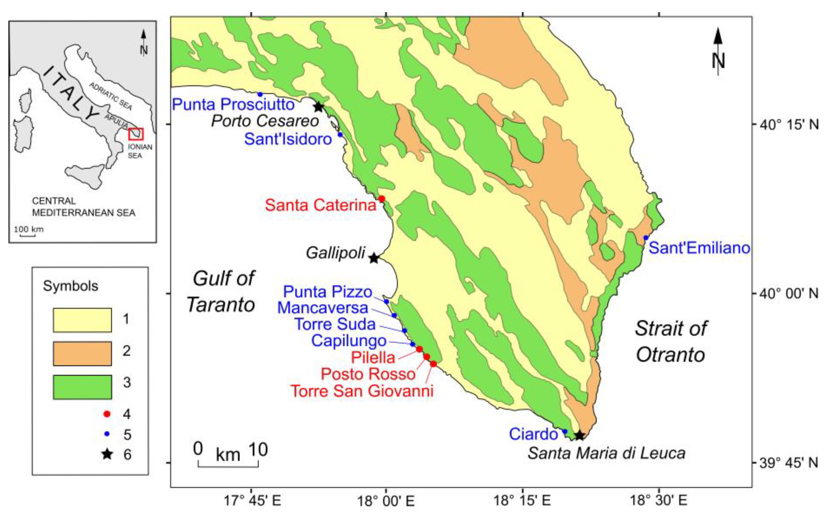
Figure 2.
Santa Caterina coast (40°08'16.93''–40°08'19.47'' N, 17°59'16.11''–17°59'21.97'' E), detection of boulder displacements; (a), (b), (d), (e) Google Earth images, eye elevation of 127 m; (c) regional aerial image; (f) transport vector of SCb boulder, eye elevation of 43 m. Blue symbols, pre-displacement position; red symbols, post-displacement position; green symbols, socket of boulder disappeared into the sea.
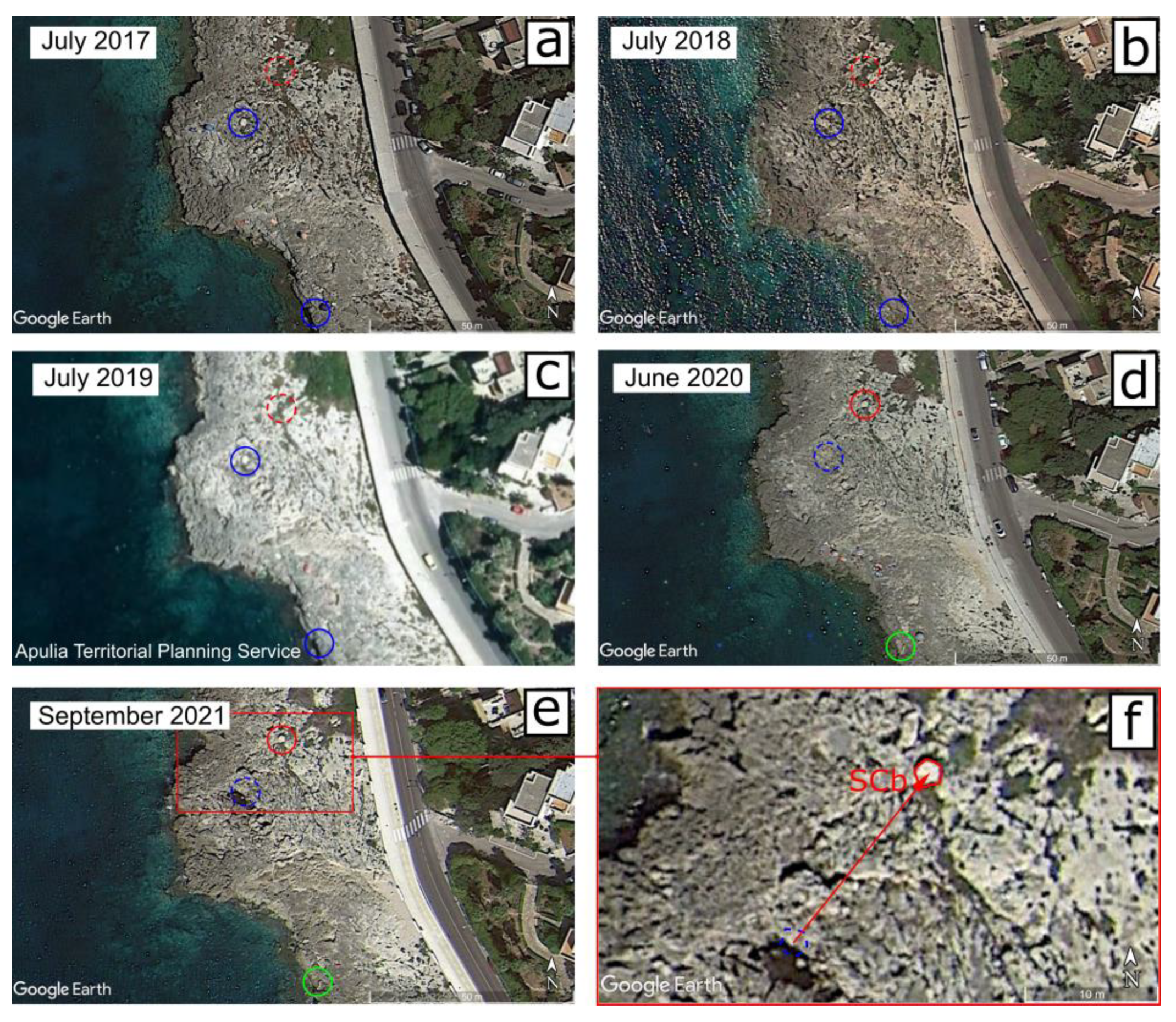
Figure 3.
Pilella coast (39°55'26.18''–39°55'27.61'' N, 18°03'25.23''–18°03'28.54'' E), detection of boulder displacements; (a), (b), (d), (e) Google Earth images, eye elevation of 73 m; (c) regional aerial image; (f) transport vector of PILm and PILn boulders, eye elevation of 38 m. Blue symbols, pre-displacement position; red symbols, post-displacement position.
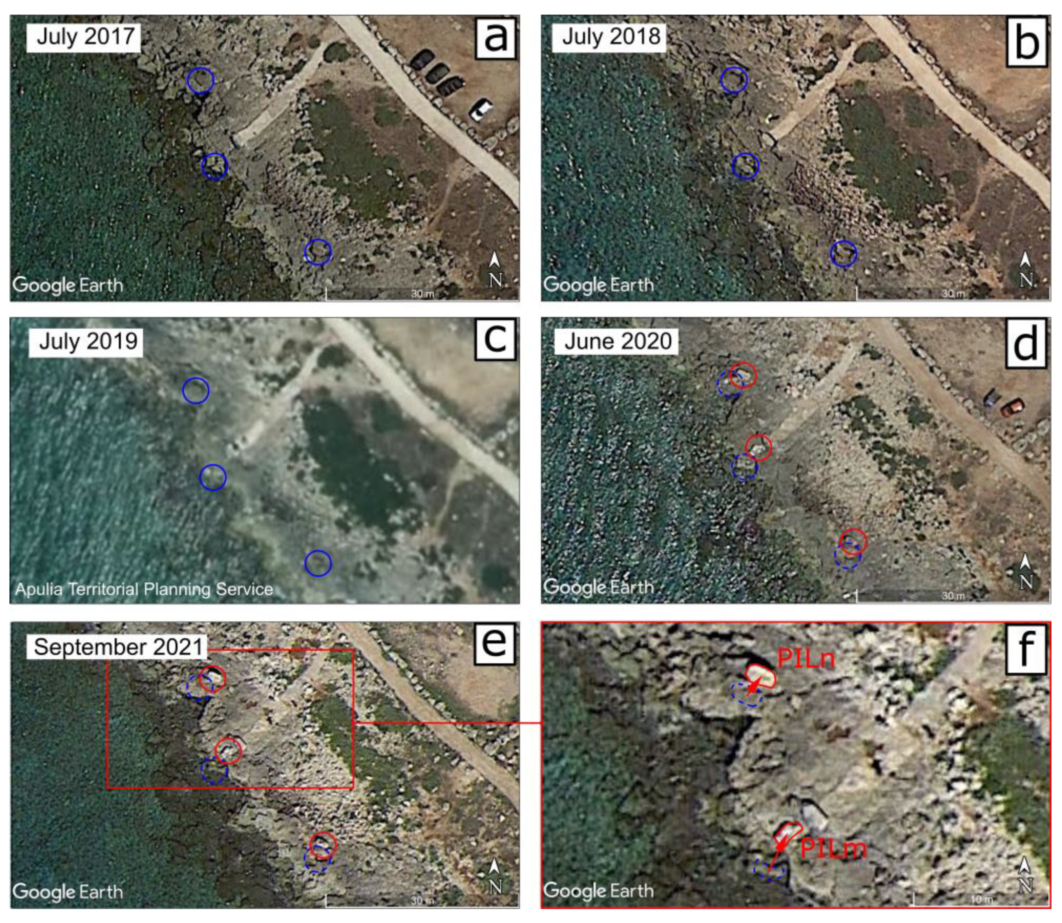
Figure 4.
Posto Rosso coast (39°54'47.70''–39°54'49.57'' N, 18°04'15.79''–18°04'20.12'' E), detection of boulder displacements; (a), (b), (d), (e) Google Earth images, eye elevation of 93 m; (c) regional aerial image; (f) transport vectors of ROf, RIi, ROj, ROk boulders, eye elevation of 35 m. Blue symbols, pre-displacement position; red symbols, post-displacement position.
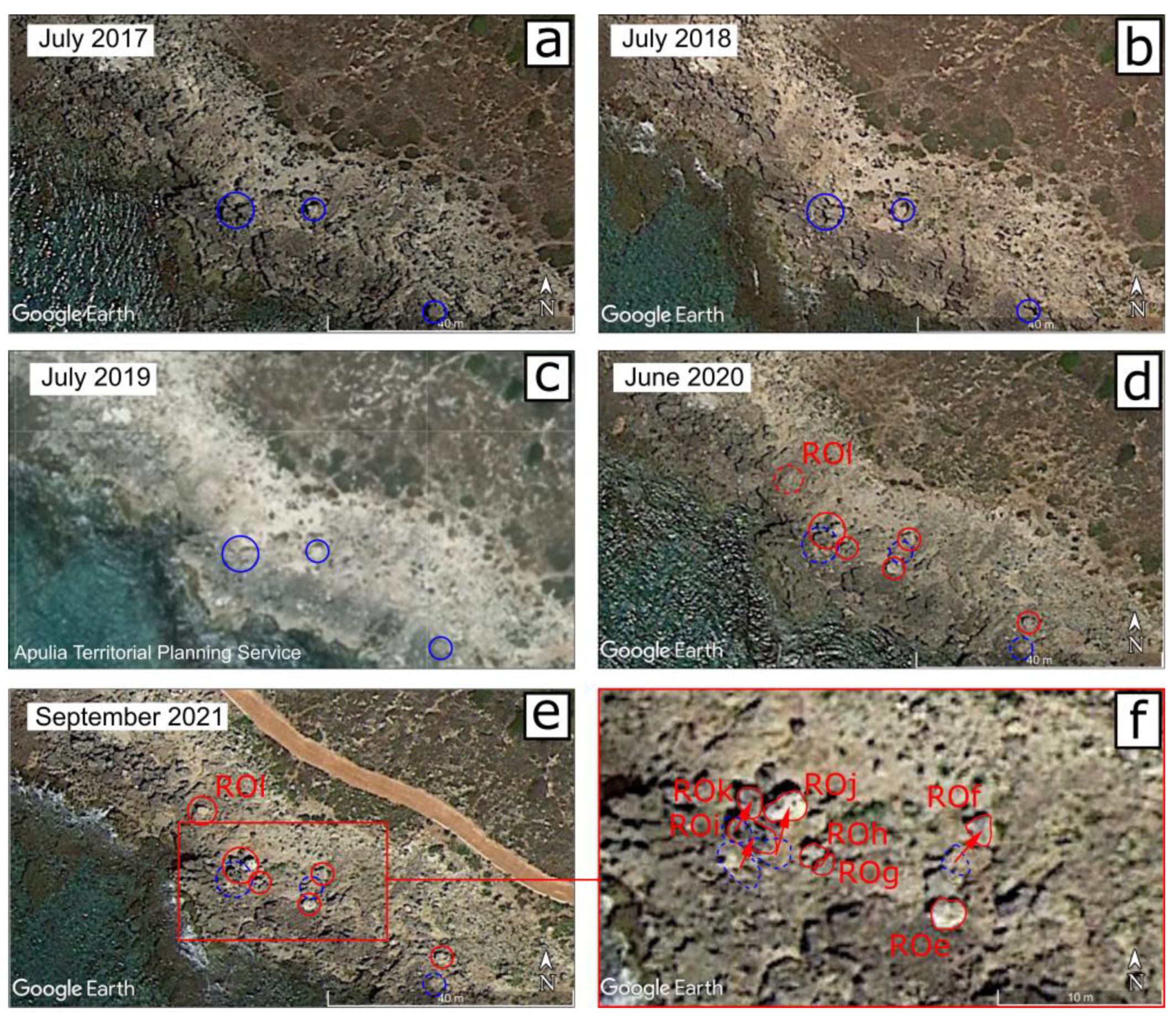
Figure 5.
Torre San Giovanni coast (39°54'03.59''–39°54'05.11'' N, 18°05'06.89''–18°05'10.90'' E), detection of boulder displacements; (a), (b), (d), (e) Google Earth images, eye elevation of 85 m; (c) regional aerial image; (f) transport vectors of SCd and SCe boulders, eye elevation of 41 m. Blue symbols, pre-displacement position; red symbols, post-displacement position.
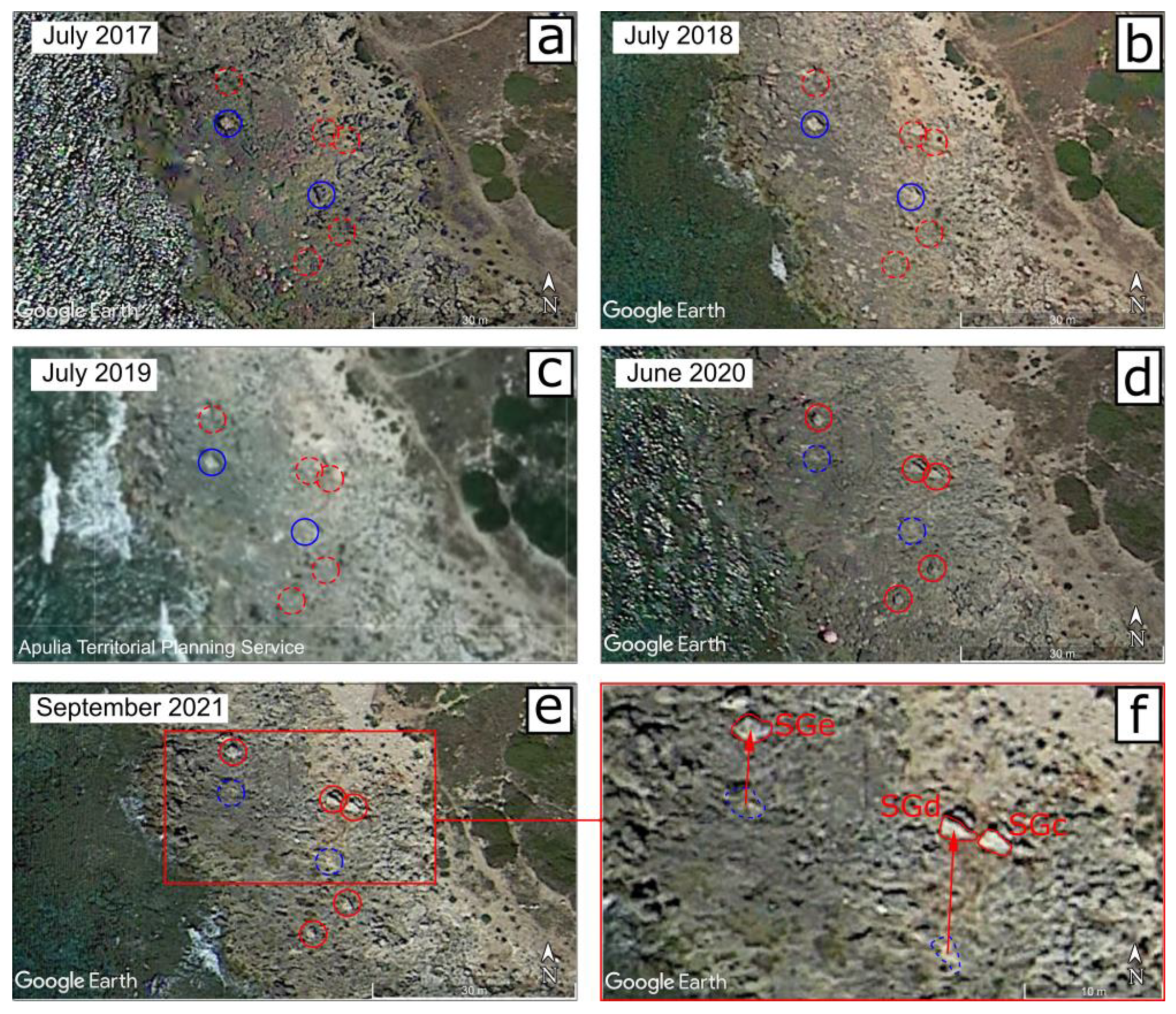
Figure 6.
Punta Prosciutto headland (40°17'32.93''–40°17'35.96'' N, 17°45'41.75''–17°45'49.46'' E), detection of boulder displacements; (a), (b), (d), (e) Google Earth images, eye elevation of 167 m; (c) regional aerial image; (f) Transport vector of PRi,j,k,l cluster, eye elevation of 35 m. Blue symbols, pre-displacement position; red symbols, post-displacement position.
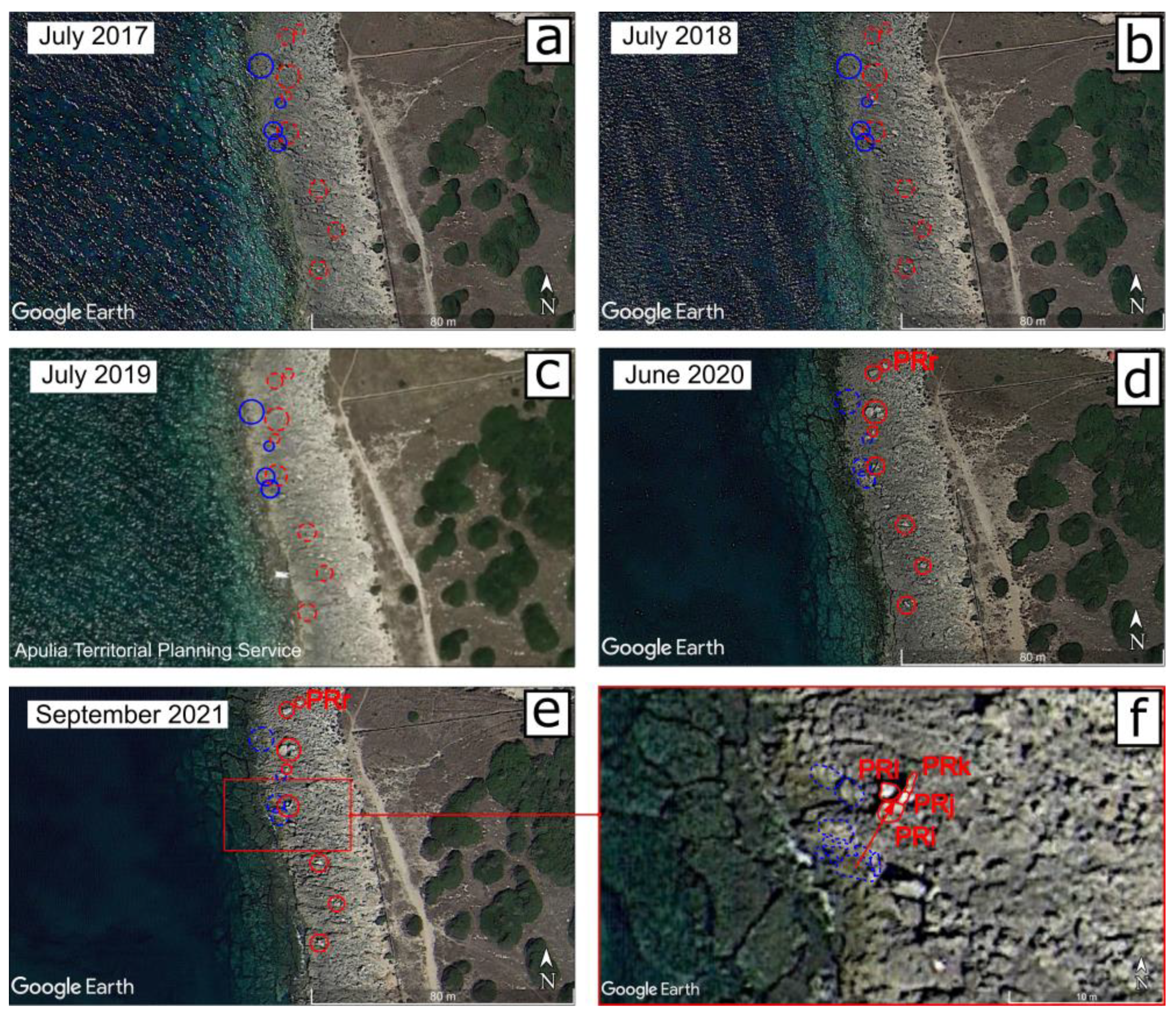
Figure 7.
Torre Suda coast (39°57'05.72''–39°57'07.66'' N, 18°01'44.75''–18°01'49.31'' E), detection of boulder displacements; (a), (b), (d), (e) Google Earth images, eye elevation of 99 m; (c) regional aerial image; (f) Transport vector of SUa boulder, eye elevation of 35 m. Blue symbols, pre-displacement position; red symbols, post-displacement position.
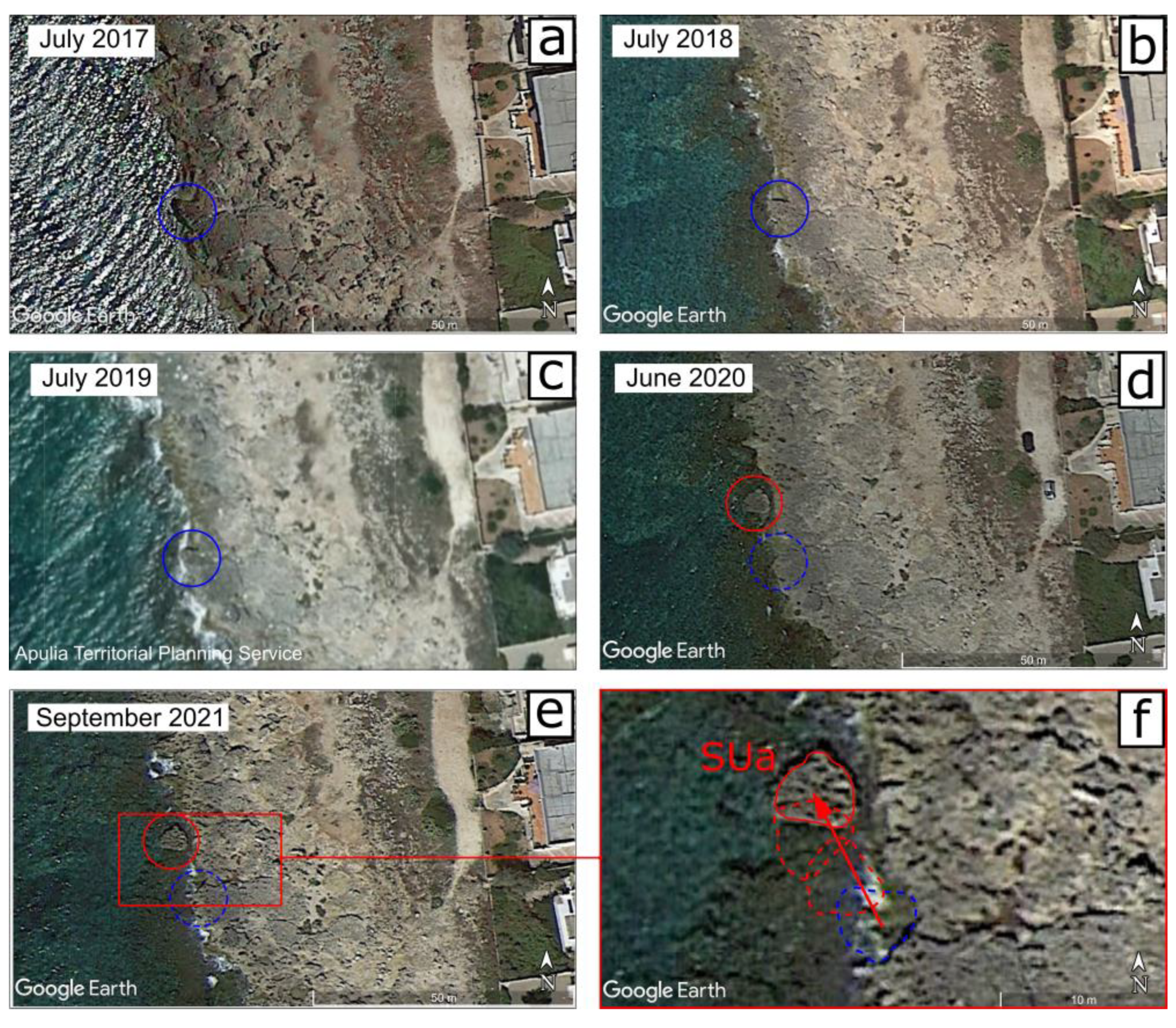
Figure 8.
Mancaversa coast (39°58'19.56''–39°58'21.50'' N, 18°00'41.53''–18°00'46.09'' E), detection of boulder displacements; (a), (b), (d), (e) Google Earth images, eye elevation of 99 m; (c) regional aerial image; (f) Transport vector of MAa boulder, eye elevation of 37 m. Blue symbols, pre-displacement position; red symbols, post-displacement position.
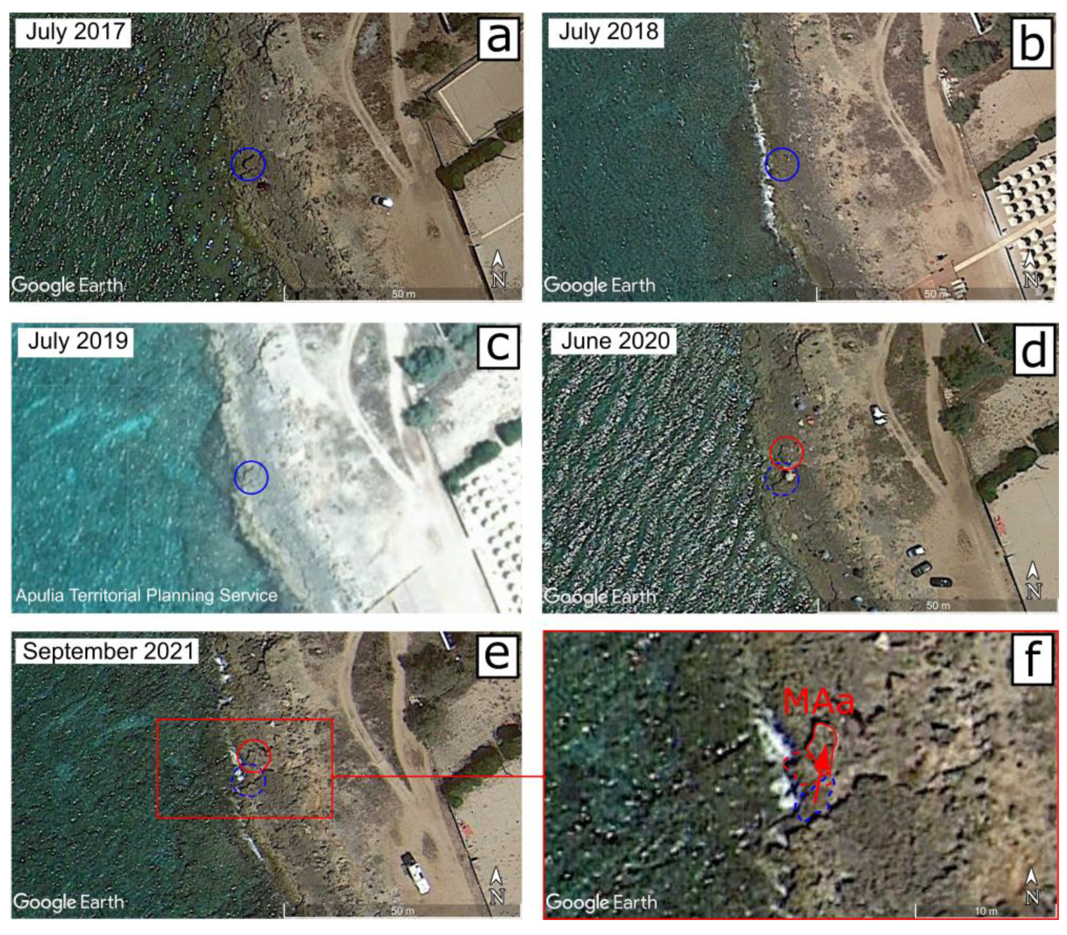
Figure 9.
Punta Pizzo coast (39°59'33.92''–39°59'35.48'' N, 17°59'45.88''–17°59'49.52'' E), detection of boulder displacements; (a), (b), (d), (e) Google Earth images, eye elevation of 80 m; (c) regional aerial image; (f) Transport vector ..., eye elevation of 35 m. Blue symbols, pre-displacement position; red symbols, post-displacement position.
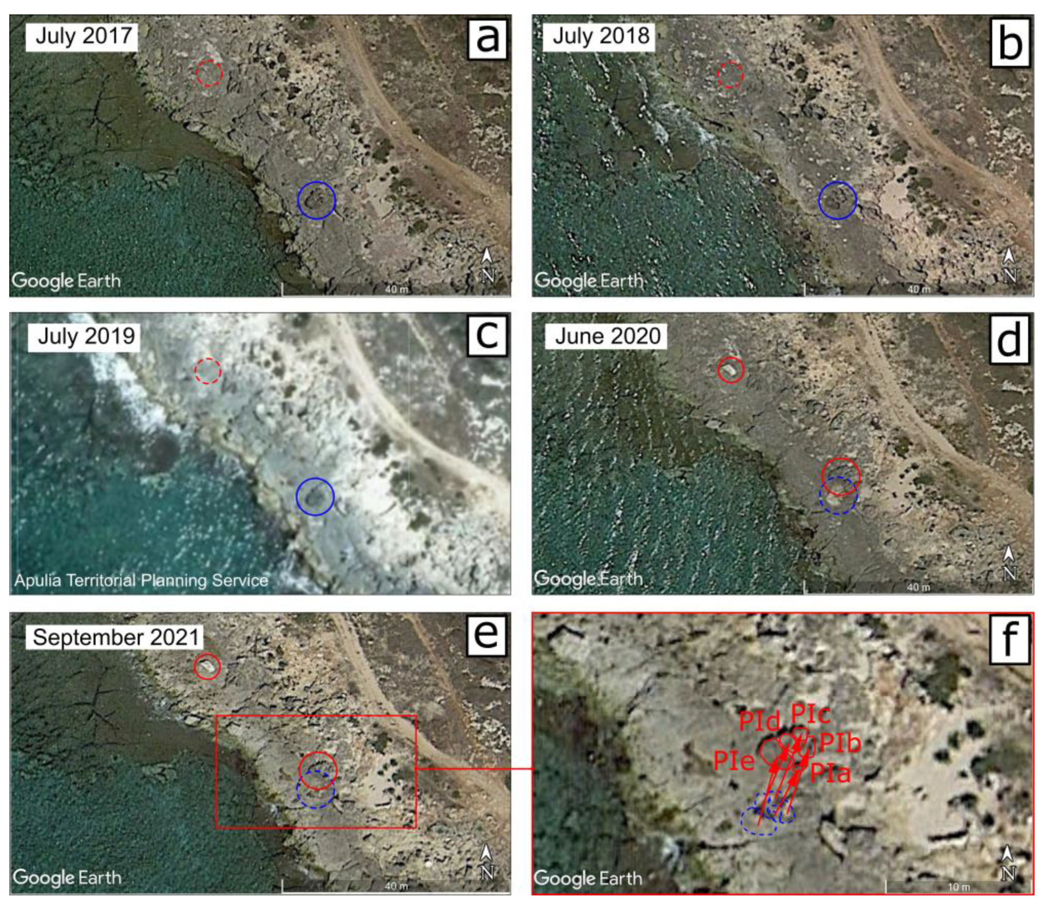
Figure 10.
Storm Power Index (in m2 h) of the storms in Table 2. Annual intervals of Table A are reported in the upper side.
Figure 10.
Storm Power Index (in m2 h) of the storms in Table 2. Annual intervals of Table A are reported in the upper side.
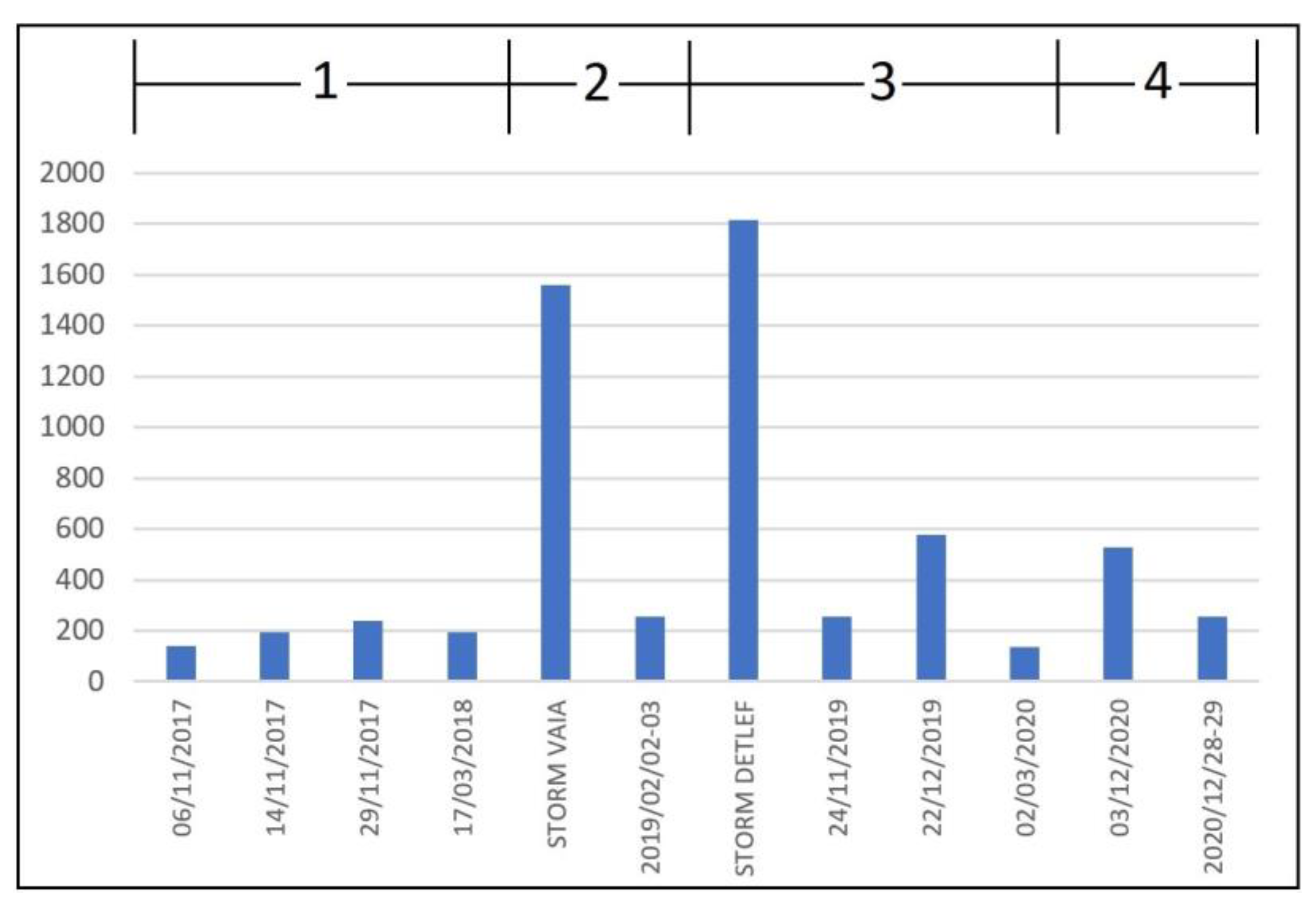
Table 1.
Acronym code (ID Code), number of identified Boulders, and number of calculated Transport Distances (No. of TD).
Table 1.
Acronym code (ID Code), number of identified Boulders, and number of calculated Transport Distances (No. of TD).
| Site Name | ID Code | Boulders | No. of TD |
|---|---|---|---|
| Santa Caterina | SC | 2 | 1 |
| Pilella | PIL | 14 | 11 |
| Posto Rosso | RO | 16 | 10 |
| Torre San Giovanni | SG | 6 | 3 |
Table 2.
Main features of the storms detected using the GLOBO-BOLAM-MOLOCH model cascade. R = Duration; F = Fetch Length; U = Wind Speed; H0 = Characteristic Wave Height. Sea State (degree, description) according to the Douglas Sea Scale.
Table 2.
Main features of the storms detected using the GLOBO-BOLAM-MOLOCH model cascade. R = Duration; F = Fetch Length; U = Wind Speed; H0 = Characteristic Wave Height. Sea State (degree, description) according to the Douglas Sea Scale.
| Days | R [h] | F [km] | U [m/s] | H0 [m] | Sea State |
|---|---|---|---|---|---|
| 2017/11/06 | 12 | 600 | 14-16 | 3.4 | 5, rough |
| 2017/11/14 | 12 | 800 | 16-18 | 4.0 | 5, rough |
| 2017/11/29 | 15 | 900 | 14-16 | 4.0 | 5, rough |
| 2018/03/17 | 12 | 700 | 16-18 | 4.0 | 5, rough |
| 2018/10/28-291 | 48 | 700 | 12-14 | 5.7 | 6, very rough |
| 2019/02/02-03 | 12 | 800 | 18-20 | 4.6 | 6, very rough |
| 2019/11/12-132 | 24 | 900 | 20-22 | 8.7 | 7, high |
| 2019/11/24 | 12 | 800 | 18-20 | 4.6 | 6, very rough |
| 2019/12/22 | 24 | 400 | 14-16 | 4.9 | 6, very rough |
| 2020/03/02 | 12 | 600 | 12-14 | 3.4 | 5, rough |
| 2020/12/03 | 18 | 600 | 16-18 | 5.4 | 6, very rough |
| 2020/12/28-29 | 12 | 600 | 18-20 | 4.6 | 6, very rough |
1 Storm Vaia; 2 Storm Detlef.
Table 3.
Minimum Flow Velocity required to set in motion the boulders.
| Boulder ID | Size (af x bf x cf) | xi | TD | PTS | MT | V | Eq. |
|---|---|---|---|---|---|---|---|
| PRq1 | 2.7 x 1.4 x 0.4 | 1.9 | 11.7 | SA | ST | 5.9 | (4) |
| SIg1 | 1.7 x 1.5 x 0.5 | 9 | 2.4 | SA | OV | 4.4 | (6) |
| SCb | 1.8 x 1.6 x 0.7 | 18.8 | 15.4 | SA | OV | 5.4 | (6) |
| PIh1 | 3.1 x 2.2 x 0.4 | 1.7 | 14.3 | SA | ST | 5.9 | (4) |
| MAa1 | 3.4 x 2.1 x 0.5 | 0.6 | 4.4 | SA | SL | 2.8 | (5) |
| SUa1 | 5.4 x 4.6 x 1.9 | 0 | 8.9 | SB | SL | 4.4 | (5) |
| CAd1 | 2.6 x 2.4 x 0.9 | 3.9 | 2.5 | SA | OV | 5.6 | (6) |
| PILj | 3.0 x 1.8 x 0.6 | 0.7 | 1.6 | SB | SL | 2.7 | (5) |
| ROd | 2.4 x 1.5 x 0.7 | 10.4 | 4.5 | SA | OV | 4.3 | (6) |
| ROn | 2.8 x 2.1 x 0.5 | 4.2 | 17.1 | SA | ST | 6.6 | (4) |
| SGe | 2.2 x 1.7 x 0.7 | 13.8 | 6.5 | SA | ST | 7.8 | (4) |
| CIc1 | 2.2 x 1.4 x 0.5 | 5.2 | 3.3 | SA | ST | 8.1 | (4) |
1 boulder detected by [11]; the MAa boulder, considered JB by [11], is here considered SA (see Appendix A).
Table 4.
Annual intervals in which the detected displacements occurred.
| CW season | No. of displacements | ||
|---|---|---|---|
| 1 | July 2017-July 2018 | 2017-2018 | 0 |
| 2 | July 2018-July 2019 | 2018-2019 | 1 |
| 3 | July 2019-June 2020 | 2019-2020 | 110 |
| 4 | June 2020-September 2021 | 2020-2021 | 2 |
Disclaimer/Publisher’s Note: The statements, opinions and data contained in all publications are solely those of the individual author(s) and contributor(s) and not of MDPI and/or the editor(s). MDPI and/or the editor(s) disclaim responsibility for any injury to people or property resulting from any ideas, methods, instructions or products referred to in the content. |
© 2023 by the authors. Licensee MDPI, Basel, Switzerland. This article is an open access article distributed under the terms and conditions of the Creative Commons Attribution (CC BY) license (http://creativecommons.org/licenses/by/4.0/).
Copyright: This open access article is published under a Creative Commons CC BY 4.0 license, which permit the free download, distribution, and reuse, provided that the author and preprint are cited in any reuse.


