
Submitted:
25 October 2023
Posted:
26 October 2023
You are already at the latest version
Abstract
TThe following three objectives were tested in this study: (1) investigate the utility of low-altitude remote sensing using UAS technology to compare the effects of different N application systems in rice production; (2) use spatial extrapolation to scale up plot-level generated to farmer field rice yield data based on crop spectral signatures, and (3) predict and map out rice productivity as a function of N placement systems. Images were captured on a UAV platform at midseason of the rice crop. Orthomosaics were developed for selected fields in rice-producing zones. Grain yields were assessed from low, medium, and high crop health plots delineated based on NDVI values. On the plot scale, UDP outyielded non-UDP by 0.84%. Individual plot yield data were scaled up to the farmer field level through Jenks natural breaks classification and es-tablishing an empirical relationship between OSAVI and plot yields. Assessment of the scaled-up field levelfield-level data also confirmed the superiority of UDP N man-agement over the non-UDP systems in promoting rice yields. Scaling up plot scale da-ta to whole field levels also facilitated generating and mapping expected yield maps for individual farmer fields in the three zones studied. This study has established a tangible simple but tangible protocol protocol for predicting and mapping rice yields in small-scale farmer fields using UAS data.
Keywords:
Unmanned Aerial Systems (UAS)
; Urea Deep Placement (UDP)
; Linear Regression
; Plot Scale
; Field Scale
; Crop Health
; NDVI
; OSAVI
; Jenks Natural Breaks Classification
1. Introduction
Rice (Oryza sativa L.) is Ghana’s second most important staple grain cereal, and it is fast becoming a cash crop for farmers in the country [1,2]. Ghana’s annual per capita rice consumption grew rapidly from 17.5 kg in 1999 – 2001 to 24 kg in 2010 - 2011 [3]. It was projected to increase to 51.63 kilograms by 2020 [4]. Rice consumption exceeds domestic production, with Ghana importing 66% of the rice it consumes. A significant factor accounting for the rice deficit is low yields. The national average is 3.28 mt ha-1 against an achievable 6.0 mt ha-1 [4]. The increasing gap between local production and rice importation can also be attributed to social, environmental, and climatic production constraints. [5]. Specifically, one can cite the high cost of improved seeds, unavailability of credit, and inadequate processing facilities. Limitations in mechanizing farming activities and low fertilizer usage also contribute to low local production. [6].
Although there has been a marginal increase in rice production to about 651,000 tons of milled rice in 2020 [4], the country is estimated to import $450 million annually to augment local demand [7]. In recent years, the Government of Ghana has prioritized developing the local rice sector with the collaboration and support of international agencies, including the United States Agency for International Development (USAID). This effort is expected to promote national rice security, youth employment, economic growth, and poverty alleviation. Research by [8] showed that applying appropriate policy measures could bridge the gap between domestic rice production and imports.
Rice requires nitrogen (N) in large quantities, making this nutrient a significant limiting factor in rice production systems. Traditionally, farmers apply N through the surface broadcast of N-containing fertilizers. However, N use efficiency (NUE) is abysmal when N fertilizers are surface broadcast. The plant’s recovery of broadcast applied N is generally between 30% - 50% [9]. Ammonia volatilization, a source of N loss, could also be as high as 50% of applied N [10,11]. Other processes leading to N losses may include denitrification, leaching, and surface runoff.
The International Fertilizer Development Center (IFDC), in collaboration with farmers, mainly from Bangladesh, developed the deep urea placement (UDP) technology [12]. The technology’s detailed description and impact are discussed [13,14]. This farmer-friendly technology improves NUE in rice production by reducing N loss through volatilization, thereby increasing output. The UDP system increases NUE by 50 - 70%, increases grain yield by 15 to 20%, and reduces fertilizer N use by 30 - 40%. Several studies have reported UDP technology’s potential for increased productivity [15]. Studies showed that UDP technology increased rice productivity by 20 - 30 %, with NUE increasing as much as 40% over conventional urea broadcasting methods [16]. As reported by [17], UDP showed a 25% savings in N fertilizer use, leading to an average 400 kg ha-1 increase in rice yield in Indonesia. Urea super granules (USG) briquette that serve as N carriers in this technology, when applied at a 56 kg N ha-1 rate, produced 25 percent higher rice grain yield than the recommended dose of 100 kg N ha-1 using the traditional broadcast of urea in Indian rice crops [18]. Similar results were obtained in Ghana and Nigeria [19,20]
Reliable and punctual estimates of hectares of rice fields and their potential production capacity are essential information for governments, planners, and decision-makers [21]. However, current national statistics on crop production capacities are often based on field surveys and farmer interviews. In addition to being inaccurate sometimes, these data acquisition methods can be extremely tedious, time-consuming, labor-intensive, and cost-ineffective. Moreover, a significant lag often exists between data collection, collation, and reporting [22].
Remote sensing has been used to monitor the status and mapping of large fields using satellite imagery. [23] used spectral reflectance data of rice fields in Taiwan from the Satellite pour l’observation de la Terre (SPOT) to develop yield prediction models. In addition to predicting rice yields, [24] used satellite data from Landsat 7, 8, and Sentinel 2 to estimate rice growth status and protein content. As intimated by [25], the relationship between vegetation index (VI) and grain yield is an important part of the N management decision tool for predicting grain yield. The VI metric has been used as an essential element in remote sensing. It is used to assess the presence and state of vegetation. It can also assess physiological state and biophysical properties variations [26], monitor crop growth, and assess vegetation stress and crop yields [27,28]. VI is based on photosynthetic responses of green vegetation to incident light. High VI, referred to in this document as “high health,” is due to high reflectance in the infrared region of the magnetic spectrum and low reflectance due to chlorophyll absorption in the red spectrum. Stressed, unhealthy, or dead vegetation manifests low VI, or “low health,” due to reduced chlorophyll pigment [29].
However, challenges to this approach include low spectral and temporal resolution and cloud cover [30]. Adding to these challenges, [31] intimated that this technology is only beneficial for large-scale studies and is inappropriate for the small-scale farming systems typical of Africa and Asia. In addition, satellites are known to have long revisit times, limiting their applications in studies requiring high-frequency image capture [32].
Over the past ten years, unmanned aerial systems (UAS) applications have expanded considerably. Unmanned platforms are more versatile and flexible than satellites or other airborne systems. Unmanned aerial vehicles (UAVs) can fly at low altitudes to acquire images of high temporal and spatial resolution [33]. These attributes make it possible to use UAS remote sensing to answer research questions and for practical applications of the technology in the field.
The normal difference vegetation index (NDVI) is derived based on light intensities reflected from canopies in the visual and near-infrared range [34,35]. This index has an enormous potential to derive information on the dynamic changes in different vegetation types. Consequently, NDVI has been a good index for investigating spatial and temporal variations in different vegetation types. However, it has been observed that NDVI saturates when estimating biomass in fully developed canopies. Other VIs have been developed to investigate spatial and temporal variations, including the optimized soil-adjusted vegetation index (OSAVI) [36] used to monitor agriculture. It has a soil adjustment coefficient (0.16) to reduce variations in soil background.
The objectives of this study are to:
(1) investigate the utility of low-altitude remote sensing using UAS technology to compare the effects of different N application systems in rice production
(2) use spatial extrapolation to scale up plot-level generated to farmer field rice yield data based on crop spectral signatures and
(3) predict and map out rice productivity as a function of N placement systems.
2. Materials and Methods
2.1. Site Characterization
This study was conducted in the Tono Irrigation Scheme (TIS) (lat. 10o 52’N; long. - 1o 11’ W). The cited scheme is in the Kassena-Nankana East District of the Upper East Region of Ghana (Figure 1a). This gravity-fed irrigation scheme is reservoir or storage-based, with a total capacity of 93 million m3 and a catchment area of 650 km2 (Figure 1b). The system has a possible 3,840 hectares of irrigable land. However, it currently supplies irrigation to 2,490 ha, which is primarily devoted to rice production. In this scheme of 4,000 smallholder producers, average farmer field sizes range from 0.2 to 0.6 ha.
2.2. Farmer volunteers and ground field mapping of producer fields
Farmer volunteers from zones H, I, and J (Figure 1b) were selected based on their N management preferences. The first group, UDP farmers, was willing to test the emerging UDP N management technology. A second group, non-UDP volunteers, was an independent group of farmers with plots within the perimeter who still needed to adopt the UDP technology. Farm operations, including land preparation, raising seedlings in nurseries, transplanting, applying fertilizers, weed, pest control, and harvesting fields, were performed independently by farmers. However, they benefited from technical support from the Irrigation Company of the Upper Region (ICOUR).
Fifty volunteers participated in this study, 25 in non-UDP and UDP N management groups, and the farmer distribution in the three zones is presented in Table 1.
Zone J had the greatest number (28) of participants. They comprised 12 (43%) non-UDP and 16 (57%) UDP volunteers. Zones H and J combined had 22 participants. Most farmers (69%) from Zone H used the UDP system, while a slight majority (56%) were non-UDP farmers in Zone I. All producers planted the locally developed AGRA rice variety.
Field sizes ranged from 0.15 - 2.7 ha, with a field average of 0.62 ha. Zone J had the biggest average field size among the three zones, with 0.86 ha. This significantly differed from 0.52 ha in Zone H and 0.4 ha in Zone I (Figure 2).
2.2. Rice fields mapping
We mapped the boundaries of each farmer’s rice field with a handheld Garmin SDSMAP 64sc global positioning system (GPS) at the beginning of the study. We used field boundary coordinates to estimate farmers’ field sizes using ArcGIS Pro. Notably, the farmer field within zones constituted the basic unit of investigation and subsequent data analysis.
2.3. UAS remote sensing and image processing
We carried out low-altitude aerial surveys of zones H, I, and J (Figure 1b) as individual units defined by boundary coordinates collected from the original ground GPS mapping. Coordinates of zones were imported into eMotion, a SenseFly software [37], to develop autonomous flight plans. Zones were surveyed using an eBee Ag, a fixed-wing UAV platform adapted with two sensors. The multispectral Sequoia contains green, red, infrared, and red-edge bands. It also contains a 16 MP RGB camera. The Sensor Optimized for Drone Applications (SODA) camera captures Red, Green, and Blue (RGB) bands. The Sequoia camera was flown at 127.4 above elevation data (AED) with 60% forelap and 80% lateral overlaps to obtain a ground resolution of 12.0 cm/pixel. The SODA camera was flown 65% forelap and 70% side-lap for a 1.6 cm/pixel ground resolution. Images were captured close to the rice crop’s booting stage.
Image processing began with the eMotion 3 software [38], which georeferenced, aligned, and stitched images together using identifiable tie points in adjacent overlapping images. Products of this process were transferred into Pix4D, in which the Standard Ag multispectral processing option was used to generate seamless high-resolution orthomosaics for Zones H, I, and J, as shown in Figure 3. These raster maps rectify heights, tilts, topographic relief, and lens distortions to ensure geometric parity [39]. Two vegetation indices were calculated, and their formulas are presented in Table 2
The regions tool isolated individual farmers’ fields identified in Figure 3 on NDVI raster maps. This step was necessary to separate vegetation indices maps for areas within individual farmer fields to avoid confounding effects from adjacent fields during subsequent analyses.
2.4. Assessment of crop health areas and rice grain determination
Three crop health areas, designated as low, medium, and high, based on NDVI values obtained from reflectance information, were identified on orthomosiacs of each farmer’s field within the three zones. A total of 141 plots were identified, with 47 plots in each health zone. These different health areas contained enough contiguous pixels to obtain 4m2 area plots. Coordinates -of the four corners defining each health plot were noted. These 4 m2 areas served as subsequent yield sampling plots. The average NDVI and OSAVI values for each 4m2 plot were also computed. At the end of the growing season, a GPS device was used to navigate to the center of each plot. A handheld sickle was used to harvest rice paddy within the sampling areas. Paddy was threshed by hand, winnowed, and weighed. The grain was air-dried for about a day, after which grain moisture content was determined using the M3GTM (Dickey-john) moisture meter. Grain weight in kg ha-1 was determined using the following formula:
Grain yield (kg ha-1) =
Grain yield (kg/net plot)*(10000/net plot)*(100-measured grain moisture content (%)
(100 – 14% standard grain moisture content)
2.5. Soil characterization
Composite surface (0 – 25 cm) soil was collected from centers of all health areas identified in farmer fields. Samples were air-dried, ground to pass a 2 mm sieve, and characterized. Particle size analysis was carried out using the pipette method [41]. A glass electrode measured soil pH in a 1:1 soil/water ratio. Organic carbon and total N were analyzed using a Leco Truspec C/N analyzer [42]. Plant available P was extracted with Bray1P solution using a 1:7 soil/solution ratio [43]. Exchangeable cations, calcium (Ca), magnesium (Mg), potassium (K), and sodium (Na), were extracted with neutral ammonium acetate (1 M NH4OAC) [44]. The concentration of cations was analyzed using ICP – AES. Cation exchange capacity (CEC) was estimated as the sum of exchangeable cations.
2.6. Yield estimation and field yield mapping based on vegetation indices
The process comprised several steps to identify the best yield predictive vegetation index for rice grain yields in non-UDP and UDP fields, as shown in Figure 4. The OSAVI was selected as the better yield predictor based on its relatively high correlation with grain yield. Second, it has no problem with saturation at high reflectance as NDVI. Using GIS-Pro, the Jenks natural breaks algorithm [45]) was used to classify the OSAVI raster ap of each isolated farmer field into the four best natural homogenous groups. According to [46], this clustering system provides the best arrangement of values into separate classes 6 in which variances within classes are minimized and maximized between groups. Compared to the 141 plots of data used in the NDVI evaluation of crop health and eventually used as a proxy for yield assessment, spatial extrapolation using the Jenks natural breaks resulted in the generation of an additional 324 points for yield evaluation. Outputs from this classification included spatial metrics such as minimum, maximum, and mean OSAVI values for each class, the spatial coverage of the class in hectares, and the percentage of the total field occupied by the health class. An empirical relationship between OSAVI values and determined plot grain yields in kg ha-1 was established to predict grain yields for the Jenks natural break classes. The predicted yield values and the number of hectares in each class were used to estimate the number of kilograms of rice grain. The sum of kilograms of grain in the four natural break classes in a field gave the total grain weight. This total weight divided by field size gave the average rice grain yield per hectare.
2.7. Statistical Analyses
Relationships between soil parameters were evaluated using Pearson correlation analysis. Analysis of variance (ANOVA) was used to test yield, and mean separations were calculated using Tukey’s studentized range with an alpha of 0.05 differences using [46]. The Shapiro-Wilk test in STATISTIX [47] was used to test the normality of the data distribution at an alpha of 0.05. Rice yield distribution in fields was evaluated using the box-and-whisker plot, a graphical, nonparametric ANOVA.
3. Results
3.1. Soil characterization
Surface (0 – 25 cm) soil was generally sandy loam in texture. The highest clay content of 18.5% occurred in Zone H (Table 3). Zone I had the highest sand content of 70.6%. This amount was significantly higher than those in zones H and J. Soils are acidic in all zones. Although not significantly different between zones, pH marginally increased from 5.4 in Zone H to 5.9 in Zone J. Zone H was inherently more fertile than Zones I and J, with higher OM, TN, and CEC levels. However, significantly high levels of plant-available P (6.58 mg kg-1) occurred in Zone J compared to 5.08 mg kg-1 and 2.32 mg kg-1in Zones I and H, respectively. Correlation analysis showed strong relationships between texture and fertility parameters (Table 3). Sand correlated negatively with pH (r = -0.478**), OM (r = -0.489**), TN (r = -0.419**) and CEC (r = -0.614**). Clay was negatively correlated with Bray P1 (r = -0.451**) but positively correlated with OM (r = 0.677**), TN (r = 0.414**), and CEC (r = 0.829**). Among the fertility parameters, Bray P1 was highly correlated with OM (r = 0.733**), while T.N. was also correlated with CEC (r = 0.501**). Although not designed, soil properties fell into two definite groups concerning N management systems. First, even though all soils are sandy loams in texture, UDP fields were significantly coarser on the surface than their non-UDP counterparts. Second, soils in the non-UDP management fields had significantly higher CEC levels (Table 3).
3.2. Orthomosaics and Crop Health Delineation
The RGB Orthomosaics were produced from imagery captured on the UAS platform. GPS coordinate boundary points were used to delineate individual farmer fields in each zone (Figure 3). The reflectance maps of NDVI and OSAVI maps generated from orthomosaics are presented in Figure 5a,b, respectively. Relationships between assigned crop health and VIs are shown in Figure 6. At this stage of rice development, OSAVI values are statistically different among the three health zones. On the other hand, NDVI values are not statistically different between the medium and high zones, but both are statistically higher than the low zone.
3.3. Midseason crop health and rice grain yield
We tested the combined grain yield data from the identified crop health areas for normality using the Shapiro-Wilk test at an alpha 0.05. The resulting W and p-values were 0.93 and 0.76, respectively, indicating a normally distributed dataset. Figure 7 shows the relationship between midseason crop health identified based on NDVI and OSAVI and grain yields. Yields from identified high-health areas were higher than medium but not statistically different. However, these two health areas produced significantly higher rice grain yields than low-health areas.
3.4. Nitrogen management systems and rice grain yields
We examined variations in rice grain yield in non-UDP and UDP N fields using the box-and-whisker plot, a graphical, nonparametric ANOVA (Figure 8). Yields from non-UDP fields were slightly more variable than those from UDP fields. Average rice grain yields ranged from 1.92 to 9.91 mt ha-1, a difference of 8.01 mt ha-1 in non-UDP fields compared to a range of 3.27 – 10.84 mt ha-1 in UDP.
The coefficient of variation in yields was 29% in non-UDP fields compared to 24.5% in UDP. Median yields in non-UDP and UDP were 6.03 and 6.77 mt ha-1, respectively. The middle 50% yield in non-UDP was between 4.94 and 7.71 mt ha-1with a difference of 2.77 mt ha-1. The UDP fields had a narrower middle 50% yield of 2.37 mt ha-1. Subsequent ANOVA showed superior grain yield under UDP N management over other N management systems used by producers (Figure 9). The average grain yield of non-UDP fields was 6.14 mt ha-1, while UDP fields yielded an average of 6.74 mt ha-1. The 9.9% difference was statistically different.
3.5. Extrapolation of yields from plot to farmer field-levels
Grain yield data from OSAVI-identified 4m2 plots were scaled to whole farmer field levels, as described earlier in the materials and methods section. The empirical relationships between OSAVI and plot rice grain yields from non-UDP and UDP fields are shown in Figure 10a,b, respectively. The predictive equations for non-UDP and UDP N treatments are given as equations 1 and 2.
Grain yield = 14.004*OSAVI – 2.5994 R2 0.3254
Grain yield = 14.278*OSAVI - 2.2194 R2 0.3633
Accompanying each prediction point were prediction intervals that express the uncertainty in the forecast when using the prediction curves.
Scaled-up plot yield data were pooled and tested for normality. The Shapiro-Wilk statistic of 0.98 and the normal probability plot confirmed the normality of non-UDP and UDP data. The box-and-whisker figure (Figure 11) showed yield ranges of 5.30 - 7.51 mt ha 8.00 mt ha-1 in non-UDP and UDP fields, respectively. Median yields were 6.08 mt ha-1 for non-UDP and 6.92 for UDP.
The ANOVA revealed that N management significantly influenced grain yield but was not zone dependent. The UDP plots produced 6.74 mt ha-1, which is significantly higher than the 6.14 mt ha-1 from non-UDP plots. (Figure 12)
At the field scale, zone*grain yield interaction was highly significant. This relationship is summarized in Figure 13. The highest average yield of 6.81 mt ha-1 from zone J is significantly higher than 6.23 mt ha-1 and 6.08 mt ha-1 in zones H and I, respectively.
3.7. Comparison of rice yields at plot and field scales
Table 4 compares the descriptive statistics of plot-level and field-scale grain yields. Comparatively, ratios of non-UDP to UDP stayed about even at plot and field scales. The table confirms the superiority of UDP N management on rice productivity over the other urea placement methods. Yield differences between UDP and non-UDP plots were 0.69 and 0.84 mt ha-1 at the plot and field scales, respectively. These yield differences were significantly different. A key observation was that grain yields assessed on health plots were highly variable in non-UDP and UDP systems. Grain yields from non-UDP fields ranged from 1.92 to 9.91 mt. ha-1. On UDP plots, the range was 3.27 - 10.84 mt. ha-1. After scaling plot yield data to field levels, yield ranges tightened to 5.50 - 7.51 mt. ha-1 and 5.63 - 8.00 mt. ha-1 tons on non-UDP and UDP fields, respectively. Furthermore, the coefficient of variation was 29 on non-UDP plots but decreased to 9.83 - on scaled-up fields. A similar coefficient of variation relationships was observed in UDP fields.
3.8. Rice grain yield mapping
Table 5 summarizes the rice grain yield potential of the three intervention zones. Zone J also had significantly higher average grain yields of 6.42 mt ha-1 and 7.17 mt ha-1 under non-UDP and UDP management, respectively. Total production for the Zone was estimated at 270.78 mt. Zone H was a distant second in all the productivity attributes. Similarly, average grain yields were 0.98 mt ha-1 higher in UDP fields than in non-UDP fields. This Zone produced an estimated total grain yield of 43.71 metric tons. Zone I had the smallest production area of 7.2 hectares and the lowest average yields in non-UDP and UDP fields, and this zone produced 3.95 mt of rice grain.
As a crucial product of this study, we developed a low resource-demanding but highly efficient methodology to produce accurate high-resolution rice yield maps as a function of the nitrogen management system, as shown in Figure 14.
4. Discussion
The study started with inventories of farmers’ N management preferences, field sizes, and the individual production fields’ soil physical and chemical characterization. The average field size was 0.8 ha, ranging from 0.15 to 2.7 ha. This finding is consistent with [48], who reported the average size of traditional rice fields in Northern Ghana as less than 1 ha.
The results of the physicochemical analysis confirmed the impoverished and variable nature of soils in this agroecological zone. The Bray P1 content ranged from 2.32 – 6.58 g kg-1, and OM levels varied from 1.16 to 1.94 g kg-1. These results corroborate the assertion of [49] that soil fertility is a severe impediment to agricultural production in the West African Savanna.
Midseason imagery captured using the UAS technology was used to generate orthomosaics. From NDVI raster maps generated from the orthomosaics, we identified low, medium, and high crop health areas within individual farmers’ fields. Results show a strong relationship between NDVI and end-of-season rice yields; however, this relationship was diminished at elevated high NDVIs. This finding agrees with [50], who also observed a non-linear relationship between NDVI, crop health, and end-of-season yields. It was asserted by [51] that NDVI saturates asymptotically as reflectance increases in dense canopies, which results in underestimating rice yields in areas with high vegetative growth. However, in this study, NDVI was sensitive enough to differentiate between N management systems, as was observed by [52].
The effect of different N placement strategies on rice grain yields was assessed at two scales: (1) NDVI-based midseason crop health plot yield data and (2) linearly extrapolated plot yields to field scales using the empirical relationship between OSAVI generated from midseason reflectance captured using UAS technology. The assessment showed the same extreme dependency of yield variability on the evaluation scale, as discussed by [53]. Grain yields within plots ranged from 1.9 - 10.84 mt ha-1 but narrowed from 5.5 to 8.0 mt ha-1 when assessed on the whole field scale. Grain yield from UDP plots was 0.69% higher than their non-UDP counterparts. At the field scale, UDP outyielded non-UDP by 0.84%. Similar relationships were obtained by [54,55] as they investigated rice yield -N placement strategies in Northern Ghana and Southern Bangladesh, respectively. Yield assessment on the field scale using the extrapolated approach also confirmed the superiority of UDP technology over non-UDP in enhancing rice yield. These findings confirm the assertion by [15,16] that UDP increases NUE by as much as 50 – 70%, increases grain yield by 15 – 20 %, and reduces fertilizer use by 30 – 40%.
While part of the study focused primarily on the impact of N management on rice grain yield, the effect of other inherent physicochemical properties became pronounced when plot yield data were scaled up to the field level for prediction. However, there were significant yield differences among zones when scaled from plot to field levels. using the scaling yields from the plot to spatial levels. The scaled-up yield data analysis shows the following relationship: Zone H>Zone J>Zone I, as shown in Figure 13. This mirrors the soil fertility trends obtained from the initial physicochemical characterization of the project site. Prominent among the fertility parameters is Bray 1P, which significantly influences rice grain yield after the N requirement is met. This is in line with a finding from a study in Pakistan (56) in which the application of 90 kilograms of P205 increased paddy rice yield by 29% over the control when the N requirement was satisfied. Moreover, Pearson correlation analysis showed a significant correlation between Bray 1P and rice grain yield. On the other hand, the low grain yield obtained in Zone I could be attributed to the relatively high level (70.6%) of sand, which could negatively impact water and nutrient relationships in the soil.
The Jenks natural breaks classification system is a data clustering system that provides the best arrangement of values rice yields in this study into separate classes in which variances within are minimized, and those between classes are maximized [57]. This system classified each isolated OSAVI reflectance raster field map into four spatially related OSAVI groups. The provided spatial statistics associated with the classification permitted estimating each field’s expected or predicted aggregated yield. The spatial distribution of predicted rice yield is presented in Figure 13.
5. Conclusions
This study demonstrates a simple but effective approach to evaluate the impact of nutrient management systems on rice productivity in small-scale production systems using UAS technology. It shows how vegetation indices obtained from UAS imagery can guide the location of plots for yield assessment. This information alone can be used as the basis to evaluate the impact of management technologies. Secondly, grain yield information collected at the plot scale level can be scaled to the farmer field levels to evaluate farmer performance. Moreover, crop yield maps can be generated at the end of the cropping season based on midseason spatial crop reflectance. The findings and outcomes of this study have practical implications at three levels: (1) As a quasi-on-farm trial, farmers became principal participants in the management of field trials, which allowed them to observe, test, and master the intricacies of the UDP technology over the traditional urea broadcasting systems. (2) Yield maps and production data are useful to local and national administrators when making food security decisions. (3) The information can be used to make tangible decisions on quantities of rice to import for local consumption in years of poor crop production. It could also be used to plan for storing and exporting rice in the hopeful seasons of sound production.
Author Contributions
Conceptualization and Methodology, A.M.1, T.L.; and V.K.A.; Field Investigation, A.M.1, T.L.; V.K.A.; A.T.D, and A.M.2; Manuscript: Original preparation, A.M.1 A.T.D; Review and Editing, V.A.K, A.M.2, R.A. All authors have read and agreed to the published version of the manuscript.
Funding
This research was carried out through the Feed the Future Technology Transfer (ATT) project, which was funded by the United States Agency for International Development (USAID). The Agronomy Department of Iowa States University funded the low-altitude activities of the study.
Conflicts of Interest
The authors declare no conflict of interest in publishing the results.
References
- MiDA (Millennium Development Authority) (2010). Investment opportunity in Ghana: Maize, Rice, and Soybean. Accra, Ghana: MiDA.
- Osei-Asare, Y. (2010). Mapping of poverty reduction strategies and policies related to rice development in Ghana. Nairobi, Kenya: Coalition for African Rice Development (CARD).
- Bannor, R.K. Long-run and short-run causality of rice consumption by urbanization and income growth in Ghana. ACADEMICIA: An International Multidisciplinary Research Journal 2015, 5, 173–189. [Google Scholar]
- Ministry of Food Agriculture (MoFA, 2021). Agriculture in Ghana: Facts and Figures (2012). Statistics, Research and Information Directorate (SRID) (pp. 1– 45). Accra.
- Denkyirah, E.K.; Aziz, A.A.; Denkyirah, E.K.; Nketiah, O.O.; Okoffo, E.D. Access to credit and constraint analysis: the case of smallholder rice farmers in Ghana. Journal of Agricultural Studies 2016, 4, 53–72. [Google Scholar] [CrossRef]
- Balasubramanian, V.; Sie, M.; Hijmans, R.J.; Otsuka, K. Increasing Rice Production in Sub-Saharan Africa: Challenges and opportunities. Advances in Agronomy 2007, 94, 55–133. [Google Scholar] [CrossRef]
- Olaf, K.; and Emmanuel, D. (2009). Global food security response: Ghana rice study. Attachment I to the Global Food Security Response West African Rice Value Chain Analysis.
- Aker, J. C.; Block, S.; Ramachandran, V.; and Timmer, C. P. (2010). West African experience with the world rice crisis, 2007-2008. The rice crisis: markets, policies and food security, 143-162.
- Ladha, J.K.; Pathak, H.; Krupnick, T.J.; Six, J.; van Kessel, C. Efficiency of fertilizer nitrogen in cereal production: retrospect and prospects. Adv. Agron. 2005, 87, 85–156. [Google Scholar]
- Alam, M.M.; Karim, R.; Ladha, J. Integrating best management practices for rice with farmers’ crop management techniques: A potential option for minimizing rice yield gap. Field Crops Research 2013, 144, 62–68. [Google Scholar] [CrossRef]
- Dong, N.M.; Brandt, K.K.; Sørensen, J.; Hung, N.N.; Hach CVan Tan, P.S.; Dalsgaard, T. Effects of alternating wetting and drying versus continuous flooding on fertilizer nitrogen fate in rice fields in the Mekong Delta, Vietnam. Soil Biology and Biochemistry 2012, 47, 166–174. [Google Scholar] [CrossRef]
- IFDC (International Fertilizer Development Center). 2013. Fertilizer deep placement. IFDC solutions. IFDC, Muscle Shoals, AL, 6.http://issuu.com/ifdcinfo/docs/fdp_8pg_final_web?e=1773260/1756718.
- Savant, N. K.; and Stangel, P. J. (1990). Deep placement of urea supergranules in transplanted rice: Principles and practices.
- Rochette, P.; Angers, D.A.; Chantigny, M.H.; Gasser, M.-O.; MacDonald, J.D.; Pelster, D.E.; Bertrand, N. Ammonia Volatilization and Nitrogen Retention: How Deep to Incorporate Urea. Journal of Environmental Quality 2013, 42, 1635–1642. [Google Scholar] [CrossRef]
- Yao, Y.; Zhang, M.; Tian, Y.; Zhao, M.; Zhang, B.; Zhao, M.; Zeng, K.; Yin, B. Urea deep placement for minimizing NH3 loss in an intensive rice cropping system. Field Crops Research 2018, 218, 254–26. [Google Scholar] [CrossRef]
- Rahman, S.; Barmon, B.K. Exploring the potential to improve energy saving and energy efficiency using fertilizer deep placement strategy in modern rice production in Bangladesh. Energy Efficiency 2015, 8, 1241–1250. [Google Scholar] [CrossRef]
- Pasandaran, E.; Gultom, B.; Adiningsih, J.S.; Apsari, H.; Rochayati, S.R. Government policy support for technology promotion and adoption: a case study of urea tablet technology in Indonesia. Nutrient cycling in Agroecosystems 1998, 53, 113–119. [Google Scholar] [CrossRef]
- Bulbule, A.V.; Purkar, J.K.; Jogdande, N.D. Management of nitrogen for rainfed transplanted rice. Crop Research-Hisar 2002, 23, 440–445. [Google Scholar]
- Shaibu aanni, A.; Adzawla, W. Effect of Urea Deep Placement Technology Adoption on the Production Frontier: Evidence from Irrigation Rice Farmers in the Northern Region of Ghana. International Journal of Biological, Biomolecular, Agricultural, Food, and Biotechnological Engineering 2017, 11, 2017. [Google Scholar]
- Liverpool-Tasie LS, O.; Adjognon, S.; Kuku-Shittu, O. Productivity effects of sustainable intensification: The case of Urea deep placement for rice production in Niger State, Nigeria. African Journal of Agricultural and Resource Economics 2015, 10, 51–63. [Google Scholar]
- Mosleh, M.K.; Hassan, Q.K.; Chowdhury, E.H. Development of a remote sensing-based rice yield forecasting model. Spanish Journal of Agricultural Research 2016, 14, e0907. [Google Scholar] [CrossRef]
- Stafford, J.V. Implementing Precision Agriculture in the 21st Century. Journal of Agricultural Engineering Research 2000, 76, 267–275. [Google Scholar] [CrossRef]
- Wang, Y.P.; Chang, K.W.; Chen, R.K.; Lo, J.C.; Shen, Y. Large-area rice yield forecasting using satellite imageries. International Journal of Applied Earth Observation and Geoinformation 2010, 12, 27–35. [Google Scholar] [CrossRef]
- Wakamori, K.; Ichikawa, D.; Oguri, N. Estimation of rice growth status, protein content and yield prediction using multi-satellite data. In Proceedings of the 2017 IEEE International Geoscience and Remote Sensing Symposium (IGARSS), Fort Worth, TX, USA; 2017; pp. 5089–5092. [Google Scholar] [CrossRef]
- Nuarsa, I.W.; Nishio, F.; Hongo, C. Rice yield estimation using Landsat ETM+ data and field observation. Journal of Agricultural Science 2012, 4, 45. [Google Scholar] [CrossRef]
- Psomiadis, E.; Dercas, N.; Dalezios, N.R.; Spyropoulos, N.V. The role of spatial and spectral resolution on the effectiveness of satellite-based vegetation indices. Proc. SPIE 9998, Remote Sensing for Agriculture, Ecosystems, and Hydrology XVIII, 99981L (25 October 2016). [CrossRef]
- Mulla, D.J. Twenty-five years of remote sensing in precision agriculture: Key advances and remaining knowledge gaps. Biosystems Engineering 2013, 4, 358–371. [Google Scholar] [CrossRef]
- Abuzar, M.; Sheffield, K.; Whitfield, D.; O’Connell, M.; McAllister, A. Comparing inter-sensor NDVI for the analysis of horticulture crops in south-eastern Australia. American Journal of Remote Sensing 2014, 2, 1–9. [Google Scholar] [CrossRef]
- Khan, Z.; Rahimi-Eichi, V.; Haefele, S.; Garnett, T.; Miklavcic, S.J. Estimation of vegetation indices for high-throughput phenotyping of wheat using aerial imaging. Plant methods 2018, 14, 1–11. [Google Scholar] [CrossRef]
- Zhang, C. H.; Kovacs, J.M. The Application of Small Unmanned Aerial Systems for Precision Agriculture: A Review. Precision Agriculture 2012, 13, 693–712. [Google Scholar] [CrossRef]
- Chapman, S.C.; Merz, T.; Chan, A.; Jakeway, P.; Hrabar, S.; Dreccer, M.F.; Jimenez-Berni, J. Pheno-copter: a low-altitude, autonomous, remote-sensing robotic helicopter for high-throughput field-based phenotyping. Agronomy 2014, 4, 279–301. [Google Scholar] [CrossRef]
- Lamb, D.W.; Brown, R.B. P.A.—Precision Agriculture. Remote-Sensing Journal of Agricultural Engineering Research 2001, 78, 117–125. [Google Scholar] [CrossRef]
- Schirrmann, M.; Giebel, A.; Gleiniger, F.; Pflanz, M.; Lentschke, J.; Dammer, K.H. Monitoring agronomic parameters of winter wheat crops with low-cost UAV imagery. Remote Sensing 2016, 8, 706. [Google Scholar] [CrossRef]
- Blackmer, T.M.; Schepers, J.S.; Varvel, G.E.; Walter-Shea, E.A. Nitrogen deficiency detection using reflected shortwave radiation from irrigated corn canopies. Agron. J. 1996, 88, 1–5. [Google Scholar] [CrossRef]
- Stone, M.L.; Solie, J.B.; Raun, W.R.; Whitney, R.W.; Taylor, S.L.; Ringer, J.D. Use of spectral radiance for correcting in-season fertilizer nitrogen deficiencies in winter wheat. Trans. Am. Soc. Agric. Eng. 1996, 39, 162. [Google Scholar] [CrossRef]
- Rondeaux, G.; Steven, M.; Baret, F. Optimization of Soil-adjusted vegetation indices. Remote Sens. Environ. 1996, 55, 95–107 http://. [Google Scholar] [CrossRef]
- 37. SenseFly. (2016). eBee:senseFly S.A. Retrieved From https://www.sensefly.com/drone/ebee-mapping-drone/.
- Mikhail, E.M.; Bethel, J.S.; McGlone, J.C. Introduction to modern photogrammetry. New York.
- Rouse, J.W.; Haas, R.H.; Schell, J.A.; Deering, D.W. (1974). Monitoring vegetation systems in the Great Plains with ERTS. NASA special publication, 351-30.
- Rondeaux, G.; Steven, M.; Baret, F. Optimization of soil-adjusted vegetation indices. Remote sensing of environment 1996, 55, 95. [Google Scholar] [CrossRef]
- Walter, N.F.; Hallberg, G.R.; Fenton, T.S. Particle size analysis by the Iowa State University Soil Survey Lab. Standard procedures for evaluation of quaternary materials in Iowa. Iowa Geological Survey, Iowa City, 1978, 61-74.
- Combs, S.M.; Nathan, M.V. Soil organic matter. p. 53–58. In. Comun. Soil Sci. Plant Anal. 1998, 22, 159–168. [Google Scholar]
- Recommended chemical soil test procedures for the north-central Sikora, L.J.; and D.E. Stott. 1996. Soil organic carbon and nitrogen. P. 157–168. In J.W. Doran and A.J. Jones (ed.) Methods for as-region. North Central Regional Res. Publ. No. 221 (revised). Mis sessing soil quality. SSSA Spec. Publ. 49. SSSA, Madison, Missouri Agric. Exp. Sta. SB 1001, Columbia, MO.
- Bray, R.H.; Kurtz, L.T. Determination of Total Organic and Available Forms of Phosphorus in Soils. Soil Science 1945, 59, 39–45. [Google Scholar] [CrossRef]
- Warncke, D.; Brown, J. R. Potassium and other basic cations. Recommended chemical soil test procedures for the North Central Region 1998, 1001, 31–33. [Google Scholar]
- Jenks, G.F. The data model concept in statistical mapping. Int. Yearb. Cartogr. 1967, 7, 186–190. [Google Scholar]
- Jenks, G.F.; Caspall, F.C. Error on choroplethic maps: definition, measurement, reduction. Ann Assoc Am Geogr. 1971, 61, 217–244. [Google Scholar] [CrossRef]
- SAS Institute Inc. 2018. SAS/STAT® 15.1 User’s Guide. Cary, NC: SAS Institute Inc Statistix 9 2019 Tallahassee FL. USA.
- Konja, T.F.; Mabe, F.N.; Alhassan, H. Technical and resource-use-efficiency among smallholder rice farmers in Northern Ghana. Cogent Food& Agriculture 2019, 5, 1. [Google Scholar] [CrossRef]
- Bationo, A.; Fening, J.O.; Kwaw, A. Assessment of soil fertility status and integrated soil fertility management in Ghana. In: Improving the profitability, sustainability, and efficiency of nutrients through site-specific fertilizer recommendations in West Africa agroecosystems; Springer, Cham. 2018; pp. 93-138. [CrossRef]
- Asrar, G.; Fuchs, M.; Kanemasu, E.T.; Hatfield, J.L. Estimating absorbed photosynthetic radiation and leaf area index from spectral reflectance in wheat. Agron Journal 1984, 76, 300. [Google Scholar] [CrossRef]
- Hobbs, T. The use of NOAA-AVHRR NDVI data to assess herbage production in the arid rangelands of Central Australia. Int. J Remote Sens 1995, 16, 1289–1302. [Google Scholar] [CrossRef]
- Rehman, T.H.; Lundy, M.E.; Linquist, B.A. Comparative Sensitivity of Vegetation Indices Measured via Proximal and Aerial Sensors for Assessing N Status and Predicting Grain Yield in Rice Cropping Systems. Remote Sensing 2022, 14, 2770. [Google Scholar] [CrossRef]
- Lin, H.; Wheeler, D.; Bell, J.; Wilding, L. Assessment of soil spatial variability at multiple scales. Ecological Modelling. 2005, 182, 271–290. [Google Scholar] [CrossRef]
- Agyin-Birikorang, S.; Tindjina, I.; Boubakary, C.; Dogbe, W. Resilient rice fertilization strategy for submergence In the Savanna agroecological zones of Northern Ghana. Journal of Plant Nutrition 2020, 43, 965–986. [Google Scholar] [CrossRef]
- Mazid Miah, M.A.; Gaihre, Y.K.; Hunter, G.; Singh, U.; Hossain, S.A. Fertilizer deep placement increases rice production: evidence from farmers’ fields in southern Bangladesh. Agronomy Journal 2016, 108, 805–812. [Google Scholar] [CrossRef]
- Khan, R.; Gurmani, A.R.; Gurmani, A.H.; Zia, M. Effect of phosphorus application on wheat and rice yield the rice-wheat system. Sarhad J. Agric. 2007, 23, 851. [Google Scholar]
Figure 1.
(a) Map showing the location of the Tono Irrigation Scheme in the Upper East Region of Ghana: (b) schematic of the reservoir serving and the perimeter and the layout of zones in the scheme.
Figure 1.
(a) Map showing the location of the Tono Irrigation Scheme in the Upper East Region of Ghana: (b) schematic of the reservoir serving and the perimeter and the layout of zones in the scheme.
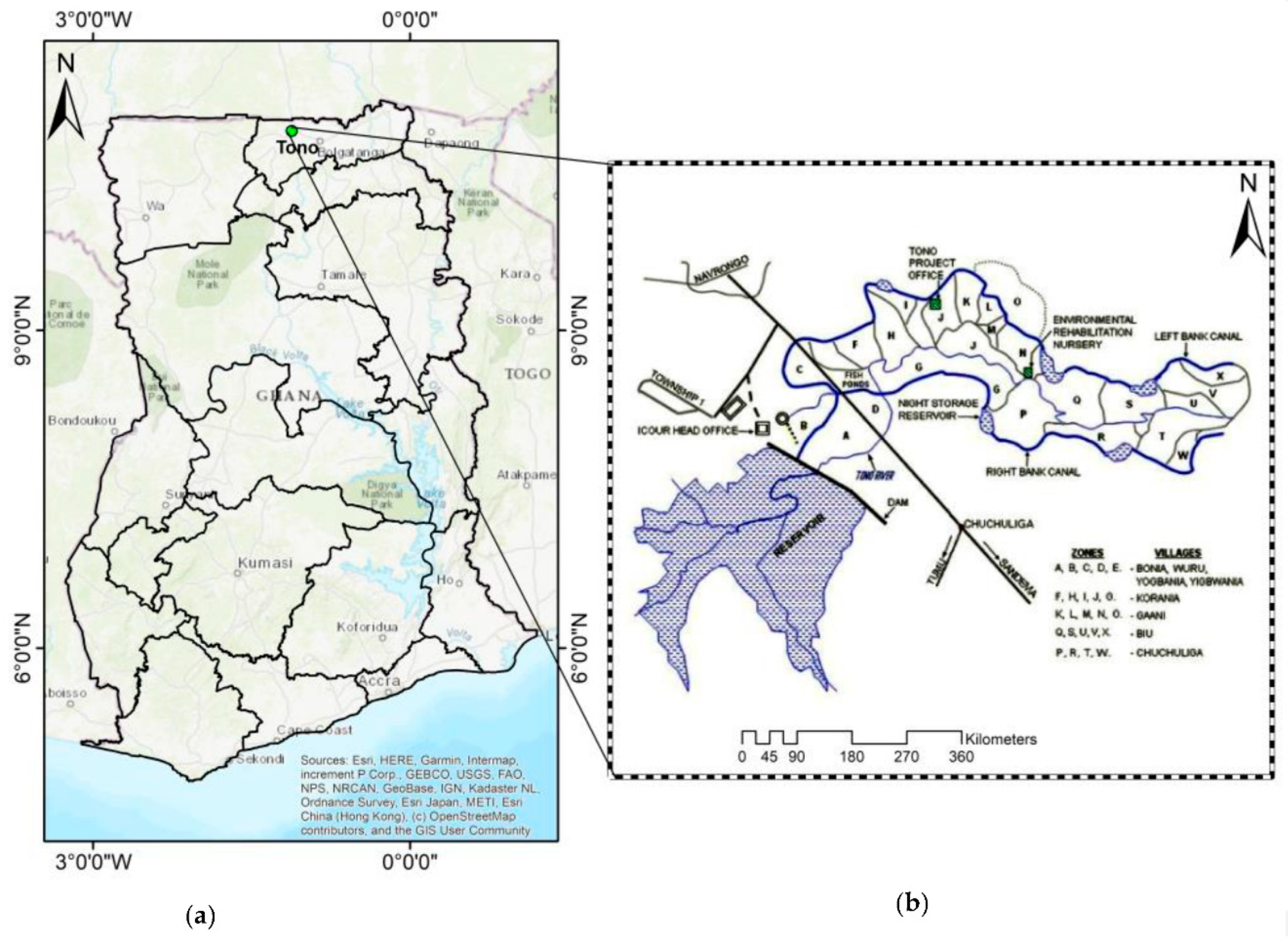
Figure 2.
Average field sizes in zones H, I, and J. columns of the same letters are not significantly different (p<0.05).
Figure 2.
Average field sizes in zones H, I, and J. columns of the same letters are not significantly different (p<0.05).
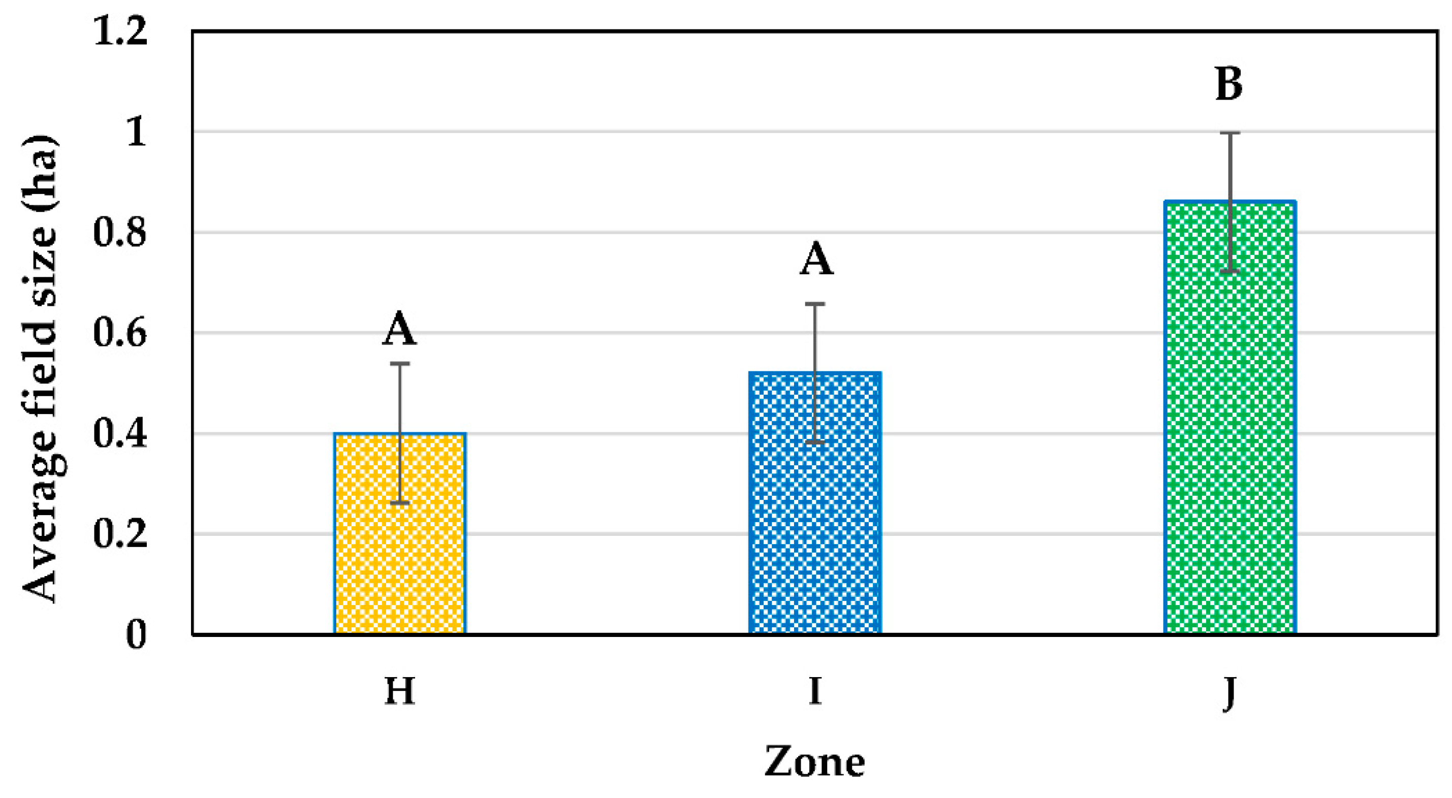
Figure 3.
R G B Orthomosaic of the study site showing mapped-out farmer field boundaries in Zone H. (yellow) , Zone I (blue), and Zone J (black).
Figure 3.
R G B Orthomosaic of the study site showing mapped-out farmer field boundaries in Zone H. (yellow) , Zone I (blue), and Zone J (black).
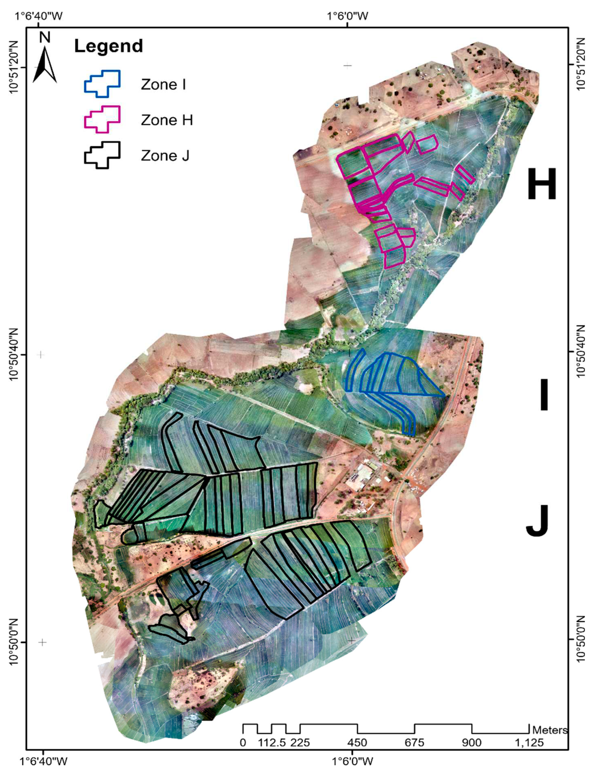
Figure 4.
Schematic workflow of activities, processes, and outputs for using UAS as an investigative tool to compare the impact of N placement on rice yields and predict and map out an end-of-season yield of rice.
Figure 4.
Schematic workflow of activities, processes, and outputs for using UAS as an investigative tool to compare the impact of N placement on rice yields and predict and map out an end-of-season yield of rice.
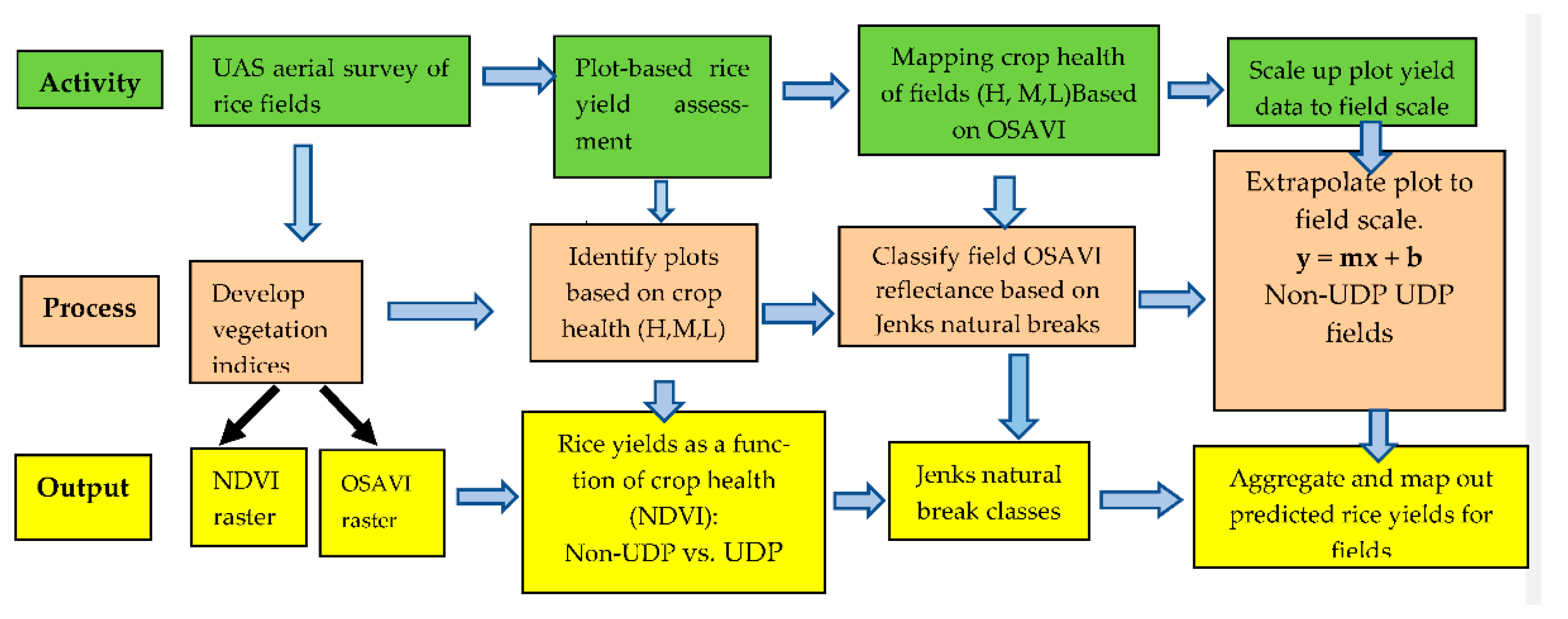
Figure 5.
Reflectance maps of (a) NDVI and (b) OSAVI of individual farmer fields in Zones H, I, and J.
Figure 5.
Reflectance maps of (a) NDVI and (b) OSAVI of individual farmer fields in Zones H, I, and J.
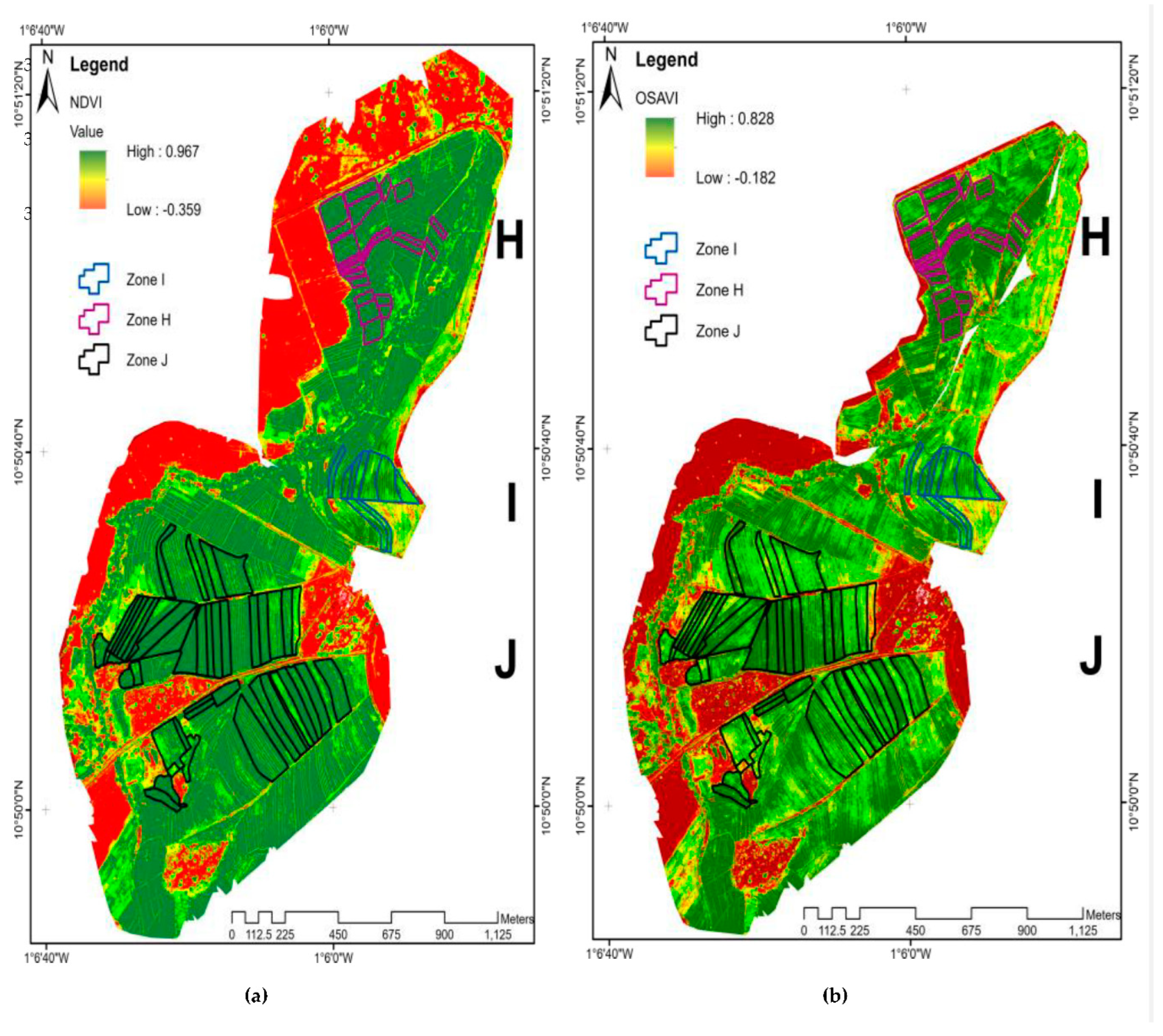
Figure 6.
Relationships between vegetation index NDVI and OSAVI) and crop health. Columns of the same color and the same letters are not significantly different (p<0.05).
Figure 6.
Relationships between vegetation index NDVI and OSAVI) and crop health. Columns of the same color and the same letters are not significantly different (p<0.05).
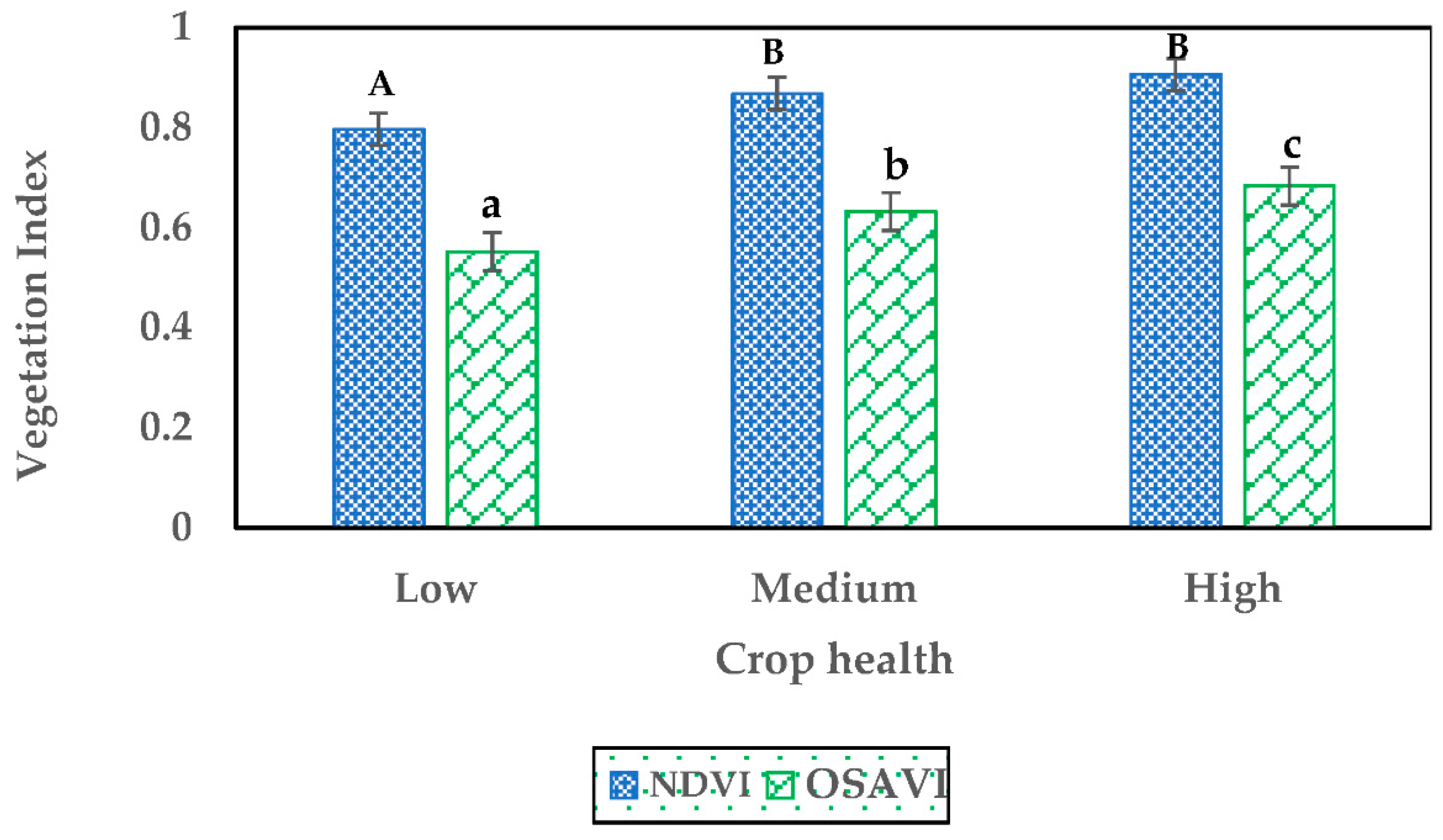
Figure 7.
Relationships between crop health as assessed by vegetation indices (NDVI and OSAVI) and grain yields. Columns of the same color and the same letters are not significantly different (p<0.05).
Figure 7.
Relationships between crop health as assessed by vegetation indices (NDVI and OSAVI) and grain yields. Columns of the same color and the same letters are not significantly different (p<0.05).
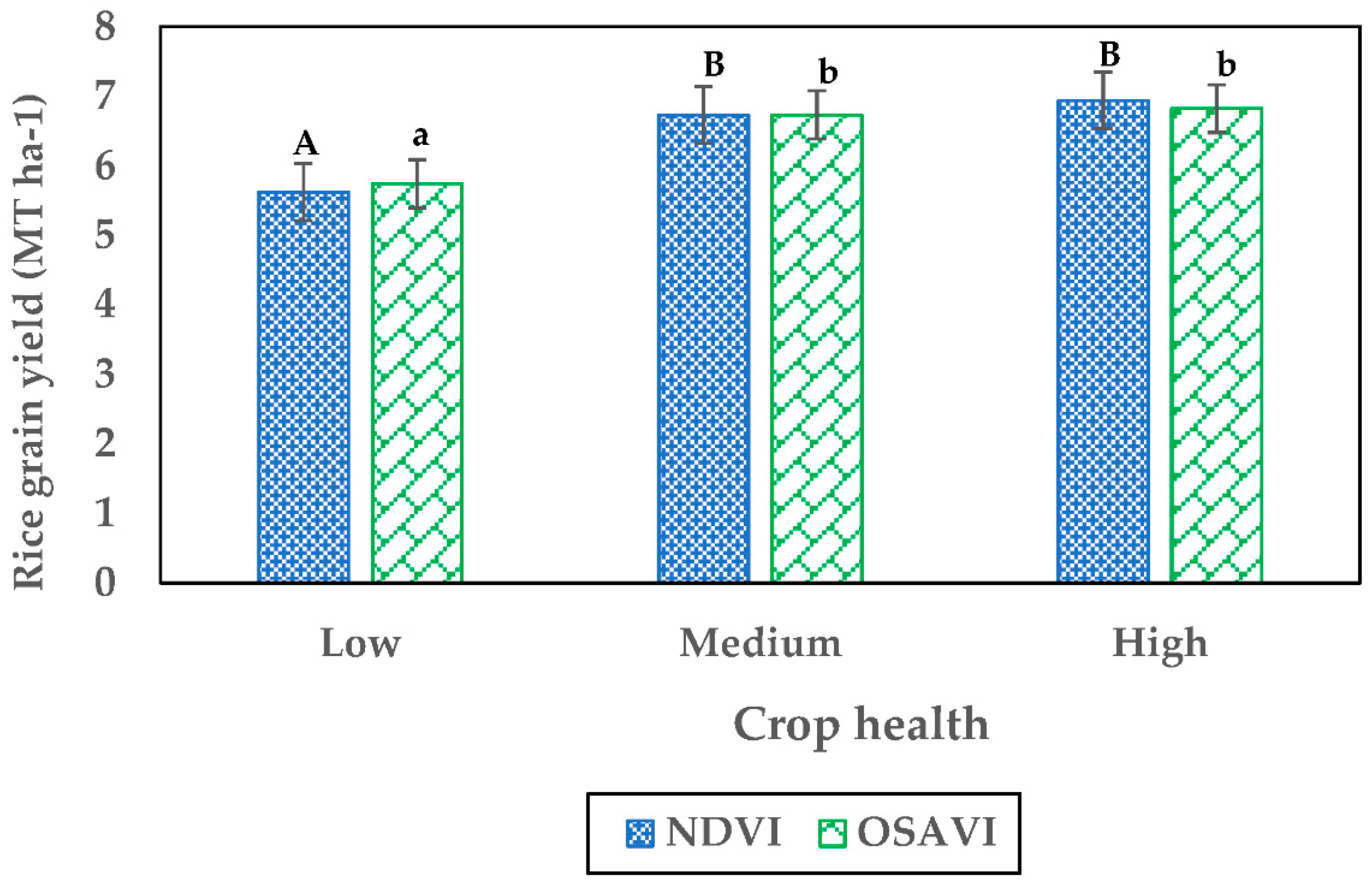
Figure 8.
Box-and-whisker plot showing variation in rice grain yields (mt ha-1) under non-UDP (n = 75) and UDP (n=68) N management systems. The figure also shows each N management system’s median, Duncan means categories and upper and lower quartiles.
Figure 8.
Box-and-whisker plot showing variation in rice grain yields (mt ha-1) under non-UDP (n = 75) and UDP (n=68) N management systems. The figure also shows each N management system’s median, Duncan means categories and upper and lower quartiles.
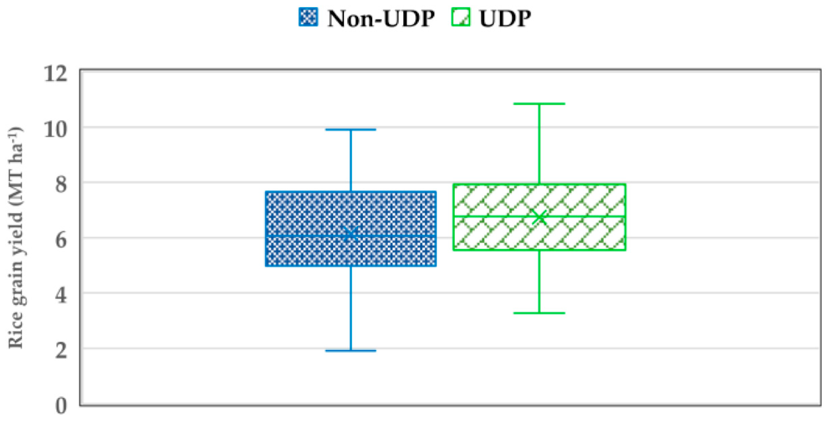
Figure 9.
Comparative assessment of average rice grain yields from non-UDP and UDP plots. Bars with the same letters are not significant at the 0.05 level.
Figure 9.
Comparative assessment of average rice grain yields from non-UDP and UDP plots. Bars with the same letters are not significant at the 0.05 level.

Figure 10.
Linear regression of rice grain yield as a function of OSAVI in (a) non-UDP and (b) UDP fields. A 95%prediction interval for each point was used for both curves to indicate that one has a 90% chance that any new observation is contained within the lower upper prediction bounds of 5 and 95%.
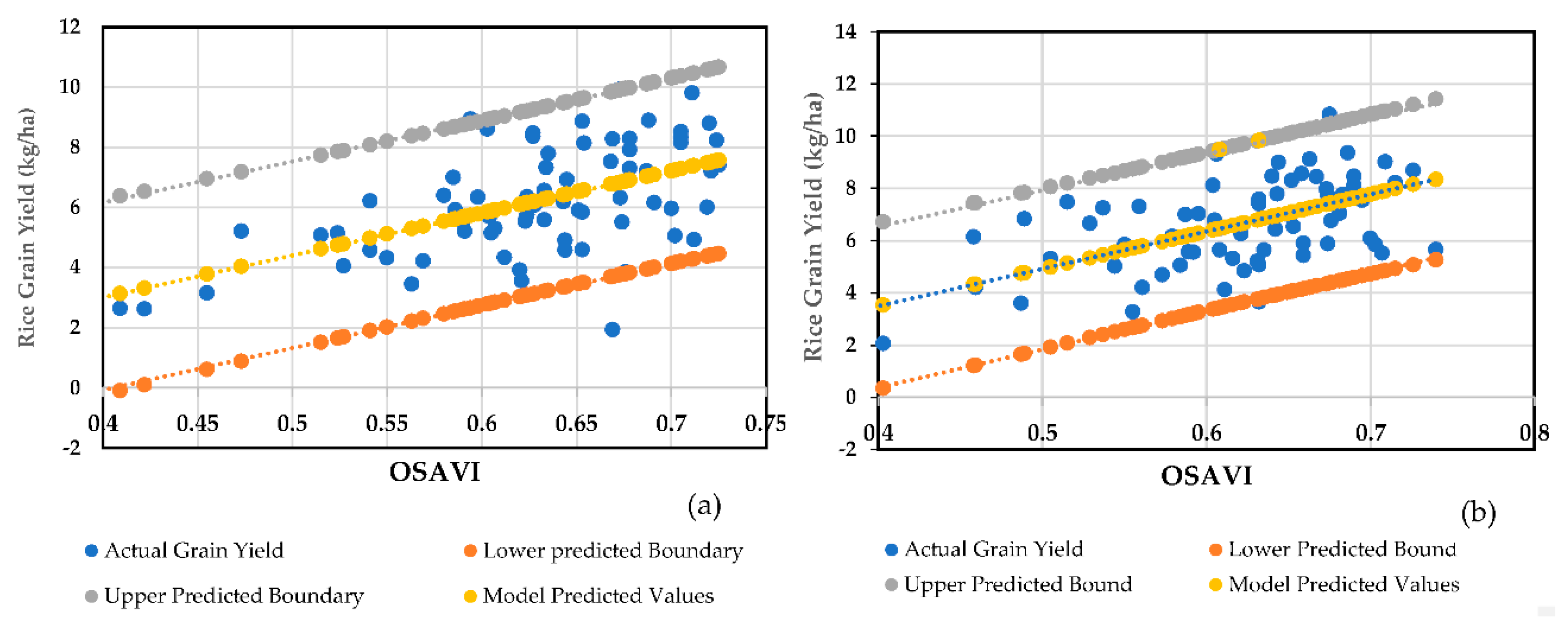
Figure 11.
The box-and-whisker plot shows rice grain yields in non-UDP and UDP fields assessed on a spatial scale. The plot shows the median, Duncan means category, median, and upper and lower quartiles.
Figure 11.
The box-and-whisker plot shows rice grain yields in non-UDP and UDP fields assessed on a spatial scale. The plot shows the median, Duncan means category, median, and upper and lower quartiles.
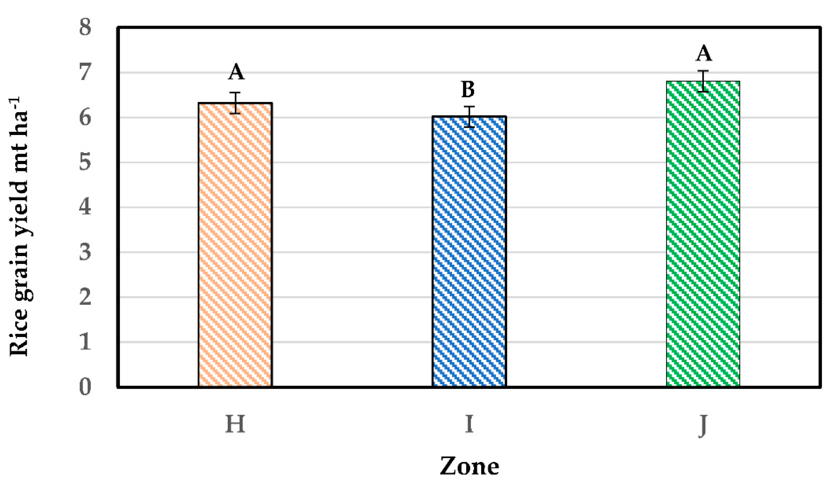
Figure 12.
Comparative assessment of average rice grain yields scaled-up non-UDP and UDP farmers’ fields. Bars with different letters are significantly different at the 0.05 level.
Figure 12.
Comparative assessment of average rice grain yields scaled-up non-UDP and UDP farmers’ fields. Bars with different letters are significantly different at the 0.05 level.
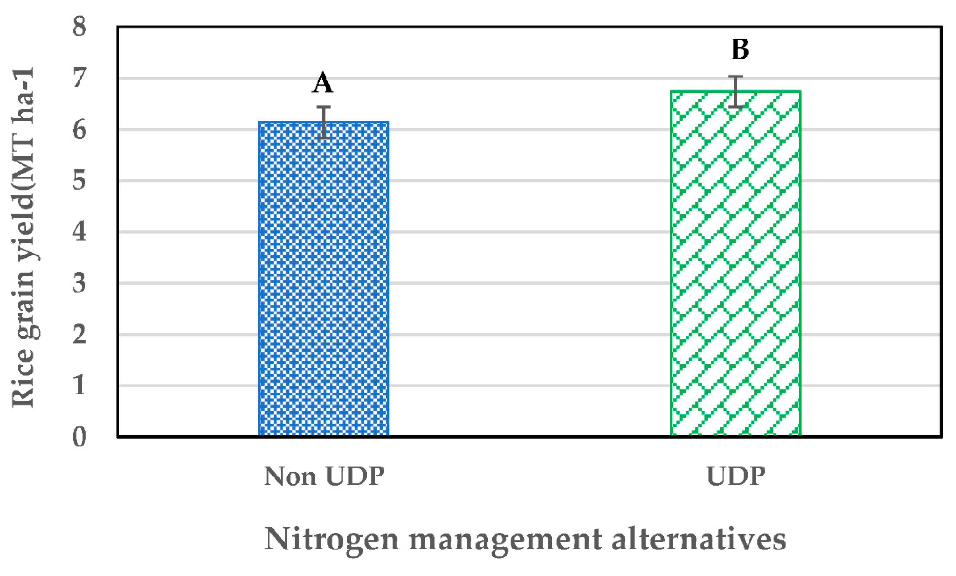
Figure 13.
Field-level rice grain yields from zones H, I, and J. Bars with different letters significantly differ at 0.05.
Figure 13.
Field-level rice grain yields from zones H, I, and J. Bars with different letters significantly differ at 0.05.
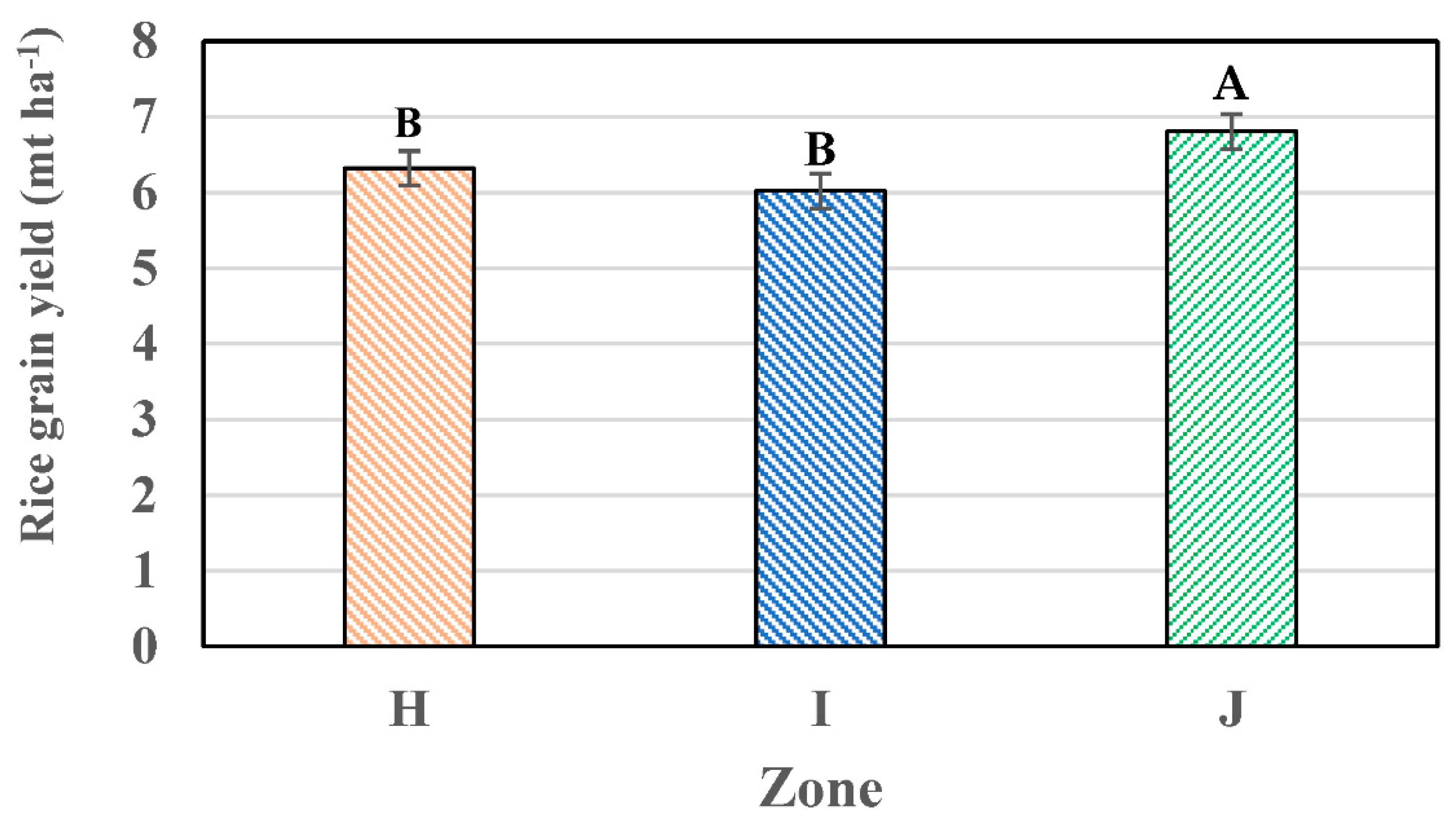
Figure 14.
Total rice grain yield in producer fields of Zones H, I, and J as a function of N management (UDP and non-UDP) systems.
Figure 14.
Total rice grain yield in producer fields of Zones H, I, and J as a function of N management (UDP and non-UDP) systems.
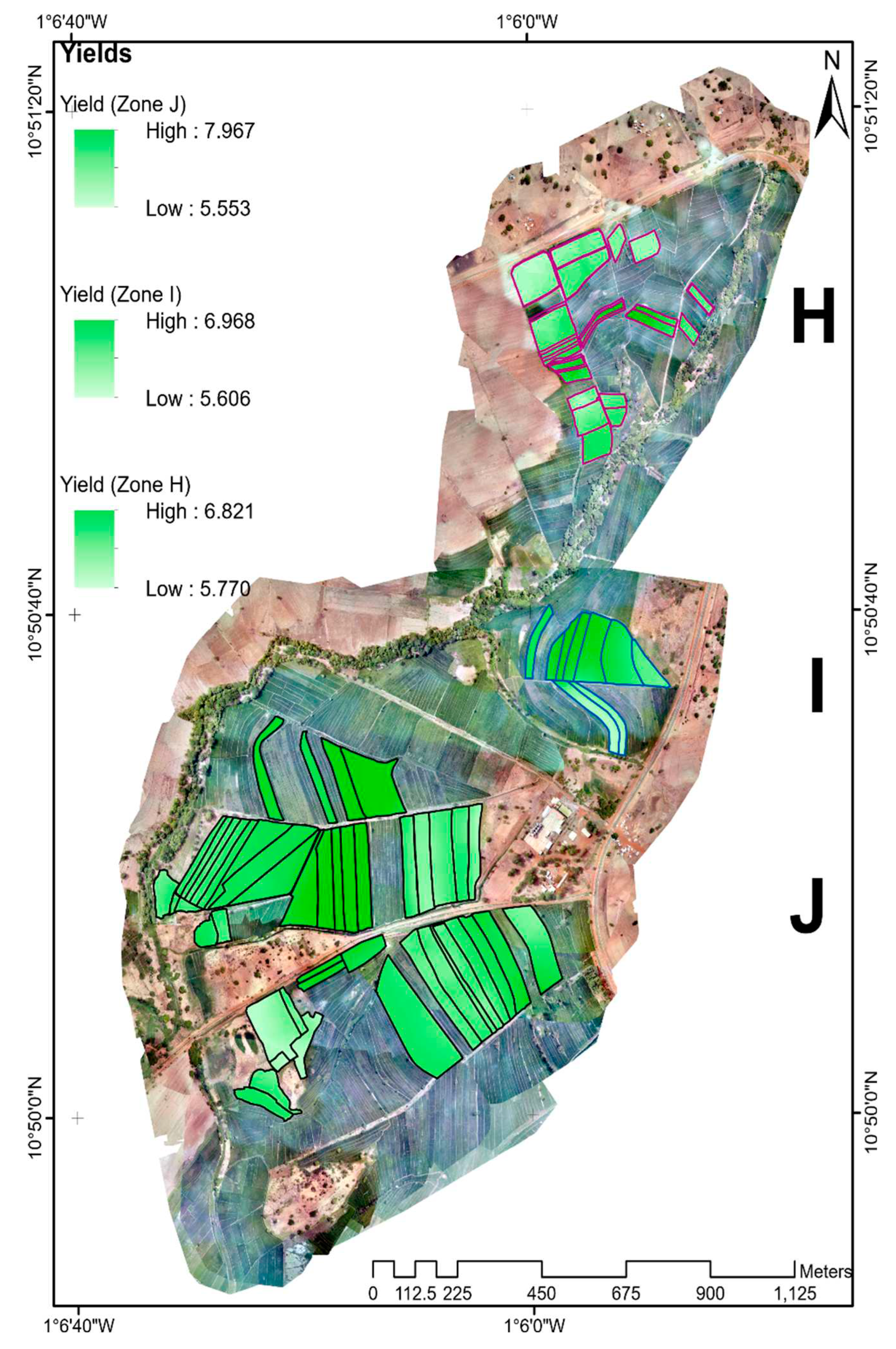

Table 1.
Volunteer Farmers and their farm size within zones H, I, and J.
| Non-UDP | UDP | |||
|---|---|---|---|---|
| Zone | Number of volunteers | Total farm size (ha) | Number of volunteers | Total farm size (ha) |
| H | 4 | 1.5 | 9 | 3.2 |
| I | 5 | 3.2 | 4 | 1.6 |
| J | 16 | 15.7 | 12 | 8.9 |
Table 2.
Vegetation indices generated from orthomosaics developed using UAS-generated data.
| Vegetation Index | Equation | Reference |
|---|---|---|
| Normal difference vegetation index (NDVI) |  |
[40] |
| Optimized Soil Adjustment Vegetation Index (OSAVI) |  |
[41] |
Table 3.
Surface soil (0 – 25 cm) properties by Zones, N management system, and their intercorrelations.
Table 3.
Surface soil (0 – 25 cm) properties by Zones, N management system, and their intercorrelations.
| Zone | Sand | Silt | Clay | pH | Bray1 P | OM | T N | CEC |
|---|---|---|---|---|---|---|---|---|
| % | mg/kg-1 % | cmol(+) kg-1 | ||||||
| Zones | ||||||||
| H | 54.7b | 27a | 18.76a | 5.4a | 5.08b | 1.94a | 0.11a | 18.38a |
| I | 70.6a | 16.7b | 13.1b | 5.7a | 2.32c | 1.16b | 0.07b | 7.48b |
| J | 56.7b | 28.7a | 14.6b | 5.9a | 6.58a | 1.23b | 0.10b | 7.94b |
| Non-UDP | 55.1a | 27.7a | 17.3a | 5.6a | 4.35a | 1.56a | 0.09a | 10.22a |
| UDP | 65.2b | 21.7b | 13.6b | 5.5a | 5.16a | 1.30a | 0.08a | 8.18b |
| Pearson’s correlation test | ||||||||
| Sand | 1 | -0.844** | -0.717** | -0.047* | 0.249 | -0.489** | -0.419* | -0.614** |
| Silt | 1 | 0.370* | -0.004 | -0.117 | 0.307* | 0.317 | 0.465** | |
| Clay | 1 | 0.136 | -0.451** | 0.677** | 0.414** | 0.829** | ||
| pH | 1 | 0.102 | -0.124 | -0.218 | 0.079 | |||
| Bray1 P | 1 | -0.177 | -0.117 | -0.417** | ||||
| OM | 1 | 0.668** | 0.733** | |||||
| TN | 1 | 0.501** | ||||||
Table 4.
Statistics of estimated rice grain yield at plot and field scales under non-UDP and UDP N management systems.
Table 4.
Statistics of estimated rice grain yield at plot and field scales under non-UDP and UDP N management systems.
| Statistic | Plot scale | Field-scale | ||
|---|---|---|---|---|
| Non-UDP | UDP | Non-UDP | UDP | |
| Average grain yield (mt ha-1) | 6.15 | 6.84** | 6.08 | 6.92** |
| Range | 1.92 – 9.91 | 3.27 – 10.84 | 5.50 – 7.51 | 5.63 – 8.00 |
| Median yield (mt ha-1) | 6.14 | 6.77 | 6.08 | 6.92 |
| Middle 50% yield ((mt ha-1) | 4.94 | 7.71 | 1.00 | 0.86 |
| Coefficient of variation | 29 | 24.5 | 9.83 | 9.86 |
Table 5.
Summary of rice productivity in Zones H, I, and J as a function of N management based on scaled-up yield data from crop health plots.
Table 5.
Summary of rice productivity in Zones H, I, and J as a function of N management based on scaled-up yield data from crop health plots.
| Non-UDP fields | UDP fields | ||||||
|---|---|---|---|---|---|---|---|
| Fields | Field size (ha) | Average grain yield (mt ha-1) | Total grain yield (mt) | Field size (ha) | Average grain yield (mt ha-1) | Total grain yield (mt) | Total zone production (mt) |
| H | 4.30 | 5.95a | 25.59 | 2.70 | 6.7ab | 18.12 | 43.71 |
| I | 2.53 | 5.82a | 14.72 | 4.70 | 6.22b | 29.23 | 43.95 |
| J | 15.52 | 6.42a | 99.64 | 23.87 | 7.17a | 171.15 | 270.78 |
Disclaimer/Publisher’s Note: The statements, opinions and data contained in all publications are solely those of the individual author(s) and contributor(s) and not of MDPI and/or the editor(s). MDPI and/or the editor(s) disclaim responsibility for any injury to people or property resulting from any ideas, methods, instructions or products referred to in the content. |
© 2023 by the authors. Licensee MDPI, Basel, Switzerland. This article is an open access article distributed under the terms and conditions of the Creative Commons Attribution (CC BY) license (http://creativecommons.org/licenses/by/4.0/).
Copyright: This open access article is published under a Creative Commons CC BY 4.0 license, which permit the free download, distribution, and reuse, provided that the author and preprint are cited in any reuse.


