1. Introduction
Neurodegenerative Diseases (NDs) are severe neurological disorders affecting millions of people worldwide with no effective treatments so far. NDs are characterized by a complex network of pathological events leading to oxidative stress, mitochondrial dysfunction, metal ion dyshomeostasis, protein misfolding, and neuroinflammation [
1]. All these factors are strongly interdependent and, although playing a key role in neurodegeneration etiology, their implications as causes or consequences have not yet been clarified. Alzheimer’s Disease (AD) accounts for 60–80% of dementia cases which are treated with few medicines available to relieve the early symptoms. The lack of treatment has led the research to evaluate as many molecules as possible, in order to discover active ingredients [
2,
3]. These preliminary screenings were carried out using in vitro neuronal models. The most useful model for such experiments is the SH-SY5Y cell line, derived from human neuroblastoma [
4,
5]. Previous studies have shown a comparison betweeen different types of neuronal models demonstrating the many advantages offered by SH-SY5Y cells: they are human–derived, do not require animal testing, they are very proliferative, and their cost of cultivation is low [
6].
AD is characterized by a slow progression, making early diagnosis difficult. Moreover, the small memory problems that characterize the early stages of AD are often misidentified as a natural consequence of aging. For these reasons, in the last years, the scientific community has put a lot of effort in the discovery of reliable biomarkers for early AD diagnosis. In this scenario, NDs need to be fully investigated combining multidisciplinary approaches for the characterization of the corresponding metabolic features. NMR metabolomics allows to identify the entire metabolite spectrum in many biological fluids and cellular extract/medium, obtaining a metabolic fingerprint (metabolic profile) that characterizes the healthy or diseased state [
7]. NMR spectroscopy, compared to other techniques, has the advantage of being rapid and not requiring a particular treatment of the samples [
8].
Data produced by spectroscopic investigations are diversified and are usually combined with multivariate statistical analysis [
9]. Indeed, one of the main problems of NMR–related tasks is the huge number of features per spectrum to be analyzed, while the available spectra often amount to small numbers. As a consequence, both dimensionality reduction and data augmentation are normally needed to automatically classify spectral data. The main technique used for the former task is Principal Component Analisys (PCA), that allows a linear dimensionality reduction. PCA is an unsupervised multivariate statistical framework based on projecting data along the most informative directions in the eigenvector space of the feature covariance matrix. While widely used, PCA may not be appropriate for complex and highly nonlinear data like NMR spectra. In fact, recent applications of Deep Learning (DL) methods to NMR data opened a new reliable path to guarantee an information–conservative feature selection [
10,
11,
12,
13].
Actually, the application of DL models to the early detection and automated classification of AD has recently gained considerable attention, as rapid progress in neuroimaging techniques has generated large–scale multimodal data [
14,
15]. Based on brain NMR images, for instance, the gray to white matter ratio can be evaluated [
16], while some forms of degeneration can be revealed, to highlight the premature brain aging typical of AD. Indeed, in the brain of AD patients, the deposition of the amyloid protein and the death of neurons, located in the gray matter, are observed. However, radiological examinations also show damage to the white matter, that part of the brain which is instead mainly made up of myelin, a substance that surrounds the neurons, facilitating their communication. In addition to deep learning techniques applied to neuroimaging, models have been implemented which are capable of integrating flexible combinations of routinely collected clinical information, including demographics, medical history, neuropsychological testing, and functional assessments [
17]. Such DL tools have been shown to often outperform the diagnostic accuracy of practicing neurologists and neuroradiologists. Finally, attention modules, able to produce saliency maps, can give rise to interpretable methods for cerebral images, showing that the detected disease–specific patterns track distinct patterns of degenerative changes throughout the brain and correspond closely with the presence of neuropathological lesions on autopsy. For the non–invasive prediction of Alzheimer’s disease, DL techniques have also been applied to retinal images [
18]. In fact, a reduction in the density of the capillary network around the center of the macula has been observed in AD patients. To early diagnose AD, retinal images were captured in different modalities (optical coherence tomography, optical coherence tomography–angiography, ultra–widefield retinal photography, and retinal autofluorescence) and integrated with patient data [
19].
In this work, we address the problem of early diagnosis of AD under a new perspective. A DL approach, alternative to PCA and based on Convolutional AutoEncoders (CAEs), is presented. A targeted procedure for NMR spectral data compression is also presented, in order to deal with the scarcity of data. Apart from the novelty inherent in the application of DL methodologies to this problem, the results of the downstream classification phase, needed for discriminating healthy and diseased cells, are very promising. To the best of our knowledge, this is the first time that such an automatic protocol has been used for the analysis of NMR spectra of SH-SY5Y cells. The rest of the paper is organized as follows.
Section 2 contains a description of the specific in vitro experiments and of the collected dataset, together with the explanation of the whole processing workflow. In
Section 3, the obtained results are presented, showing the advantage of using a DL approach instead of PCA for data dimensionality reduction. Finally,
Section 4 collects some conclusions and traces future perspectives.
2. Materials and Methods
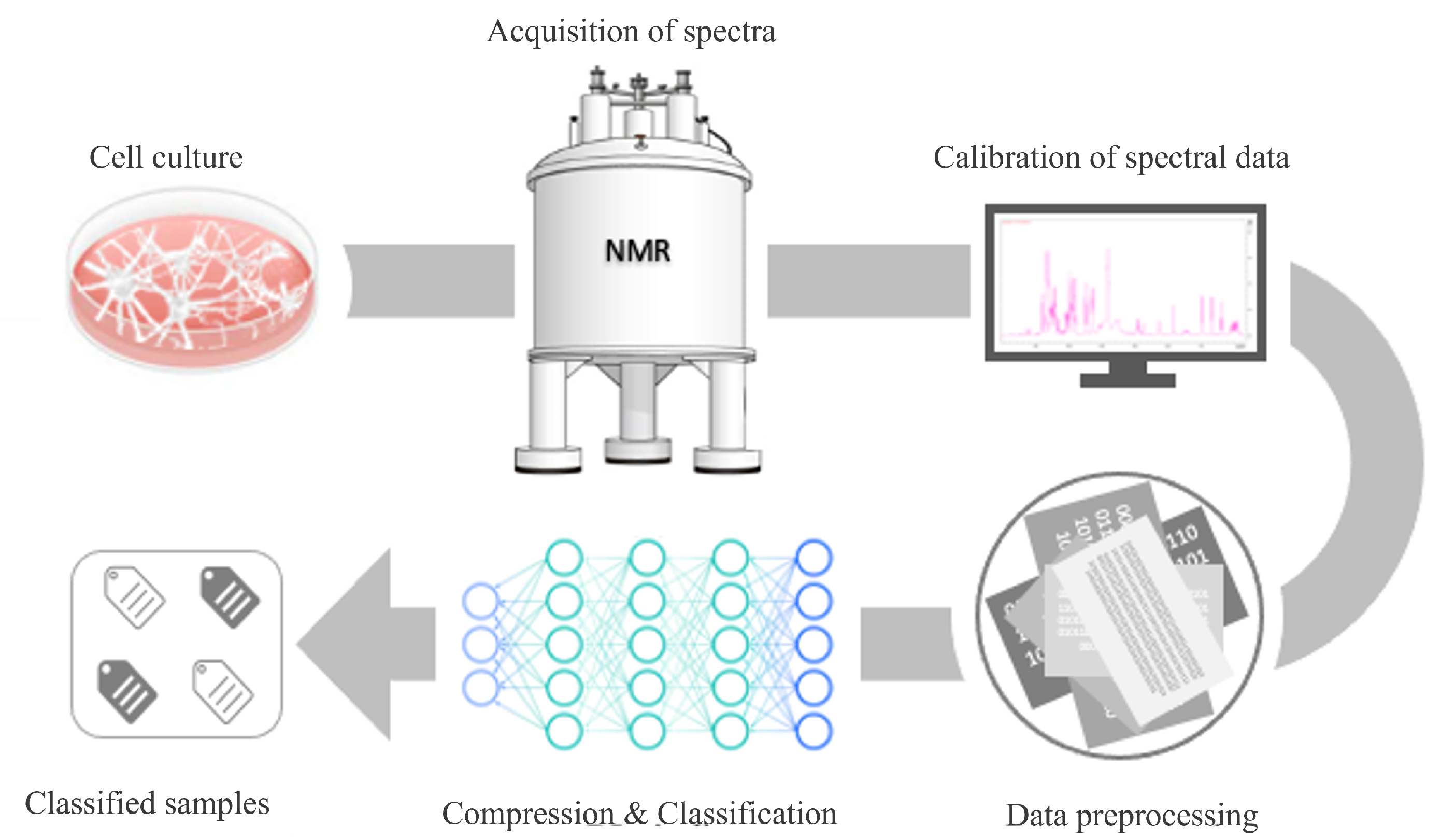
In this section, we focus first on the wet lab experimental setting used to obtain our dataset, from the cell culture to the NMR spectroscopical analysis of the metabolite content of the cells. Then, the collected dataset of spectra is described. Finally, we present the DL method used to embed the NMR spectra and to classify them — as related to healthy or diseased cells — and the evaluation metrics. The key steps of the approach used in this study are schematically represented in
Figure 1.
2.1. NMR experiments
The NMR samples analyzed in this work were obtained by collecting the cellular media of differentiated SH-SY5Y neuroblast–like cells treated with different concentrations of several compounds, including the peptide Amyloid
1–42 and the galantamine and lycorine alkaloids. The cellular experiments were performed according to the procedure reported in [
20]. The cellular vitality, determined by the Neutral Red Uptake (NRU) test, was strongly dependent on the type of the applied treatment. Each cellular experiment was executed on biological triplicates. 1mL of the growth medium related to each experiment was collected for the metabolomics analysis and stored at
until the registration of 1H NMR spectra. Frozen samples were thawed at room temperature and shaken before use.
of
containing
TMSP was added to
of each sample. The mixtures were homogenized by vortexing for
and transferred into 5 mm NMR tubes for the analysis. The pH of each sample was controlled and adjusted to the value of
for all the NMR tubes. All the 1H NMR spectra were recorded with a Bruker Avance III 600 MHz spectrometer (Bruker BioSpin) operating at controlled temperature (
) and equipped with a
BBI probe with a z–axis gradient coil and an automatic tuning–matching (ATM). The spectra of the growth media were acquired with a 1D Nuclear Overhauser Enhancement Spectroscopy (NOESY) presaturation pulse sequence, 128 scans,
data points, a spectral width of
and a relaxation delay of
. The raw data were multiplied by exponential line broadening before applying the Fourier transform. Transformed spectra were automatically corrected for phase and baseline distortions and calibrated using TopSpin 3.6.4 (Bruker Biospin srl).
2.2. Dataset preparation
The collected dataset is composed of 94 spectra of metabolites from healthy and diseased cells — with 55 healthy and 39 diseased patterns. Moreover, a
percentage vitality is attached to each sample, representing the cell health status. According to the literature [
21,
22], a sample is considered cytotoxic if the percentage vitality value is smaller than 70%. Hence the vitality threshold is set to 70%.
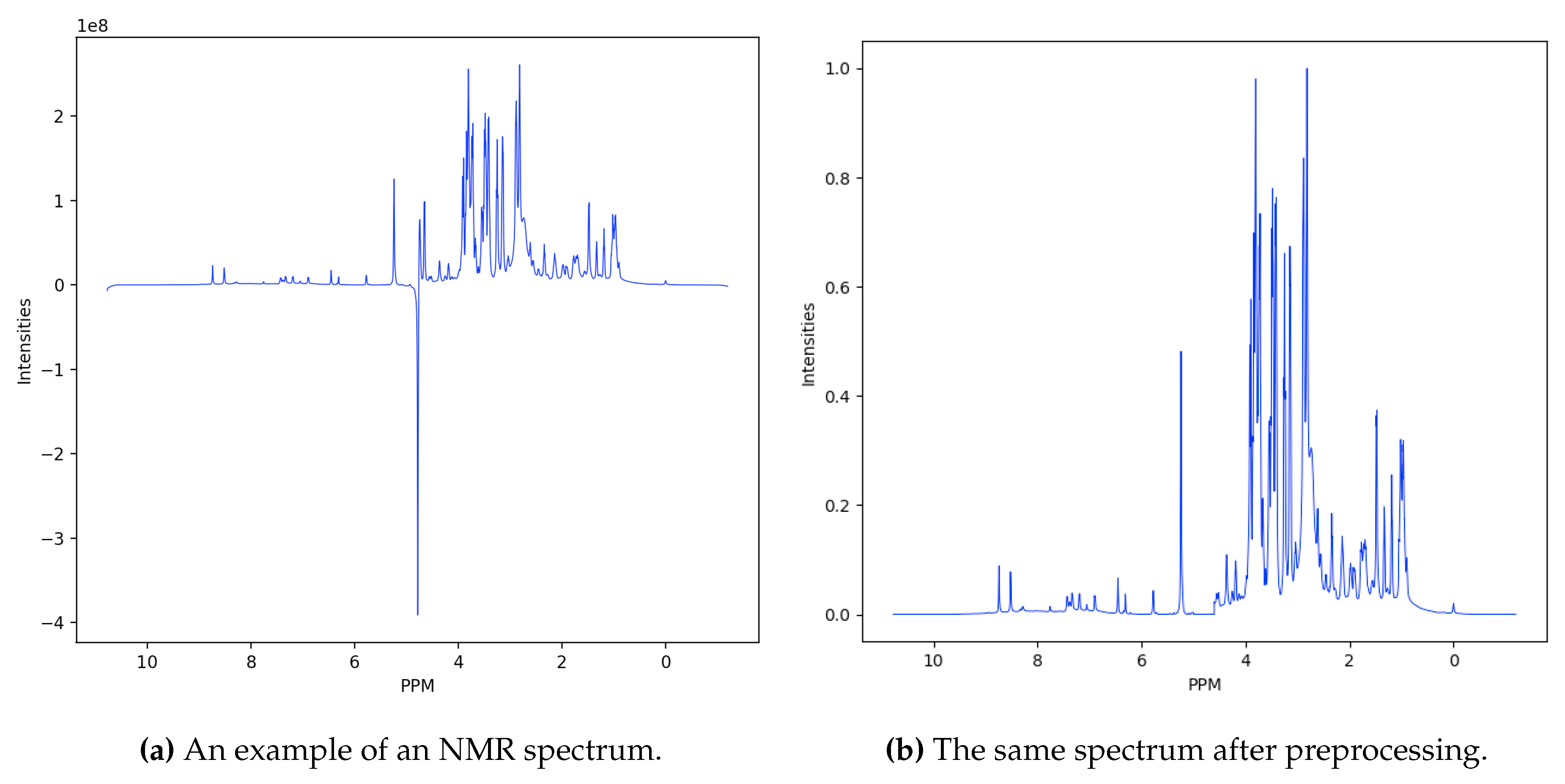
Data are represented as sequences of ppm (parts per million) intensities, with each spectrum described by
intensity values (see
Figure 2a, for an example). The first preprocessing step consists in filtering the spectra, setting zero values in the sequence elements corresponding to intensities between 4.6 and 5 ppm — which are consistent with water molecules —, and greater than 9 or less than −0.5 ppm, corresponding to the head and the tail of the spectra, respectively. While the head and the tail must be filtered out because they collect noisy data, the water region has a very high signal coming from the hydrogen atoms, spanning all the metabolite spectrum. Excluding the first and the last zero values, each sequence is constituted by
intensity values. Finally, the intensity values are normalized in the range
(see
Figure 2b).
Finally, in order to obtain an adequate number of examples to train the DL model used for data compression, each original spectrum was split into 44 sub–spectra, with length . In practice, a dataset of samples was obtained, 80% of which ( samples) was used for training while the remaining 20% (828) constituted the test set.
2.3. Processing pipeline
The considered task is a binary classification problem made difficult by both the scarcity of data and their high dimension. For this reason, our approach is based on two main phases: the reduction of the size of the feature vectors and the classification. Reducing the size of the spectra decreases the computational cost (in terms of the number of parameters to optimize) of the classification model. Dimensionality reduction is commonly done using linear methods, such as PCA or LDA; however, in this document, AutoEncoders (AEs) have been chosen, because they are nonlinear and learnable, while PCA is used as a baseline. Instead, some support vector machines (SVM), with different kernels, have been applied for classification.
2.3.1. Autoencoders
AEs [
23,
24] are unsupervised (actually,
self–supervised) models able to learn compressed representations, or
embeddings, of the input data in their inner layer. They have been used in various applications, e.g. for dimensionality reduction [
25], anomaly detection [
26,
27], and sample generation [
28,
29,
30]. Their structure consists of two modules, an
encoder and a
decoder. The encoder performs a dimensionality reduction of the input, producing its
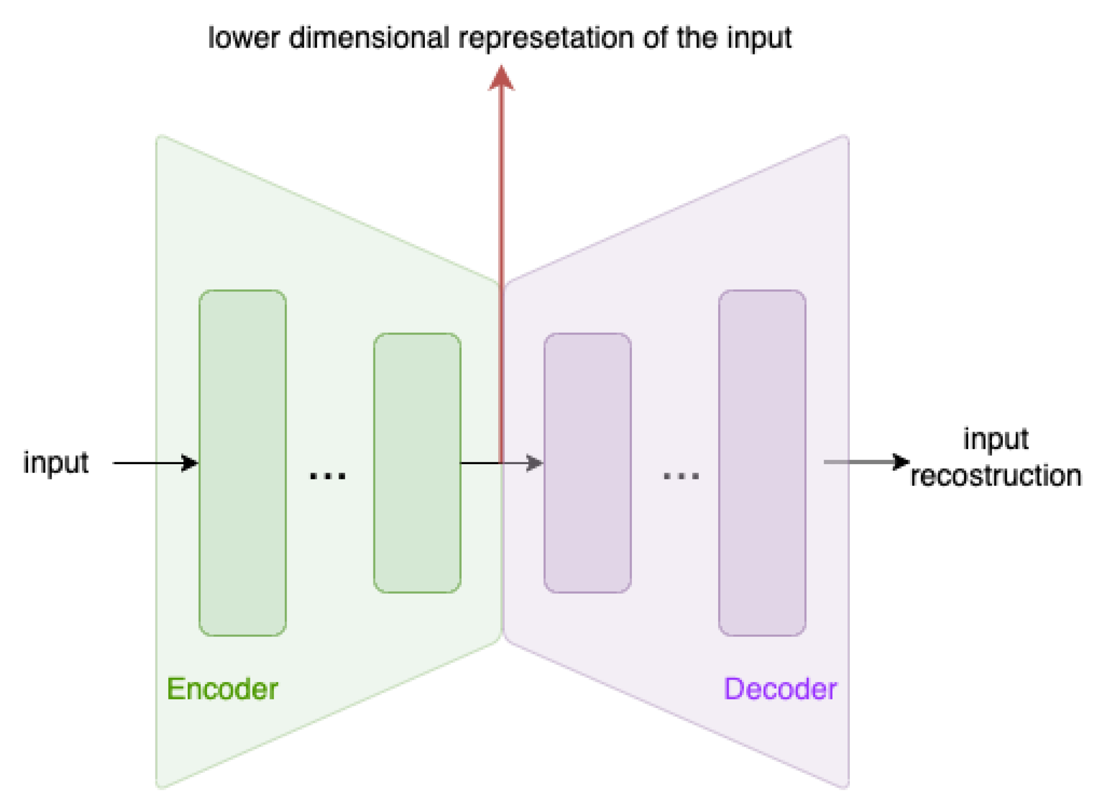
latent space representation, while the decoder re–expands the latent representation into the original dimension, so that, using the input data as targets, a reconstruction of the input can be obtained. The autoencoder architecture is shown in
Figure 3. Usually, both the encoder and the decoder are MultyLayer Perceptrons (MLPs). However, in this work, we have also employed one–dimensional Convolutional AutoEncoders (1D–CAEs), where the two modules are realized by a pool of one–dimensional convolutional layers (due to the sequential nature of the input data).
A similar model was proposed in Wang
et al. [
31] to compress ECG signals. Nevertheless, to the best of our knowledge, this is the first time that AEs have been applied for NMR spectral data embedding.
In our experiments, we have employed both MLP–AEs and 1D–CAEs, changing the encoder — and, consequently, the decoder — architecture with respect to the number of layers, of neurons per layer, and, for CAEs, the filter and kernel size. In particular, for the encoder of MLP–AEs, 2 or 3 dense layers with
ReLU activation are considered, the first one composed by
neurons, while the number of neurons in the last layer varies in
. The middle layer (when present) has a fixed dimension equal to
. It is worth noting that, if 16 neurons are used for representing each sub–spectrum in the latent space, then each spectrum is embedded into a vector of dimension 704 (
). The 1D–CAE architectures have instead 3, 4 or 5 layers in the encoder, with kernel size 7 and stride 5 for the first 4 layers, and kernel size 7 and stride 2 for the last layer. By changing the number of filters, compressed spectra with 4 or 8 channels were obtained.
Table 1 collects the hyperparameters that define all the AE architectures used in the experiments. The values for the convolutional hyperparameters were set based on a grid search procedure aimed at optimizing the compression performance.
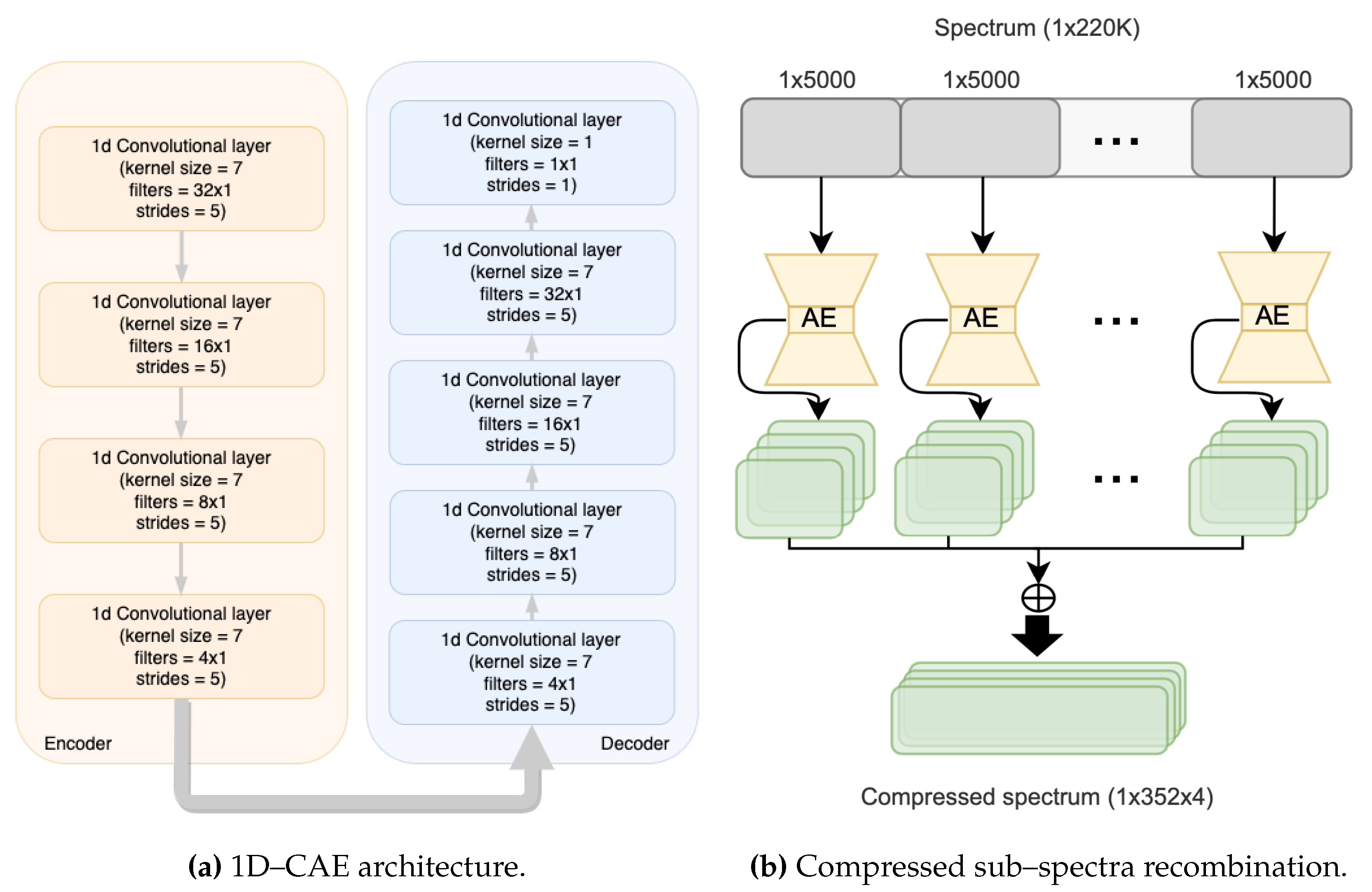
Finally,
Figure 4a shows, as an example, the best performing 1D–CAE architecture, composed of 4 layers of 1D convolutional blocks with a decreasing number of filters per layer, from 32 to 4, kernel dimension equal to 7, and stride equal to 5.
Figure 4b depicts how the outputs of the 1D–CAEs are combined to reconstruct the full compressed spectrum from the sub–spectra.
2.3.2. PCA
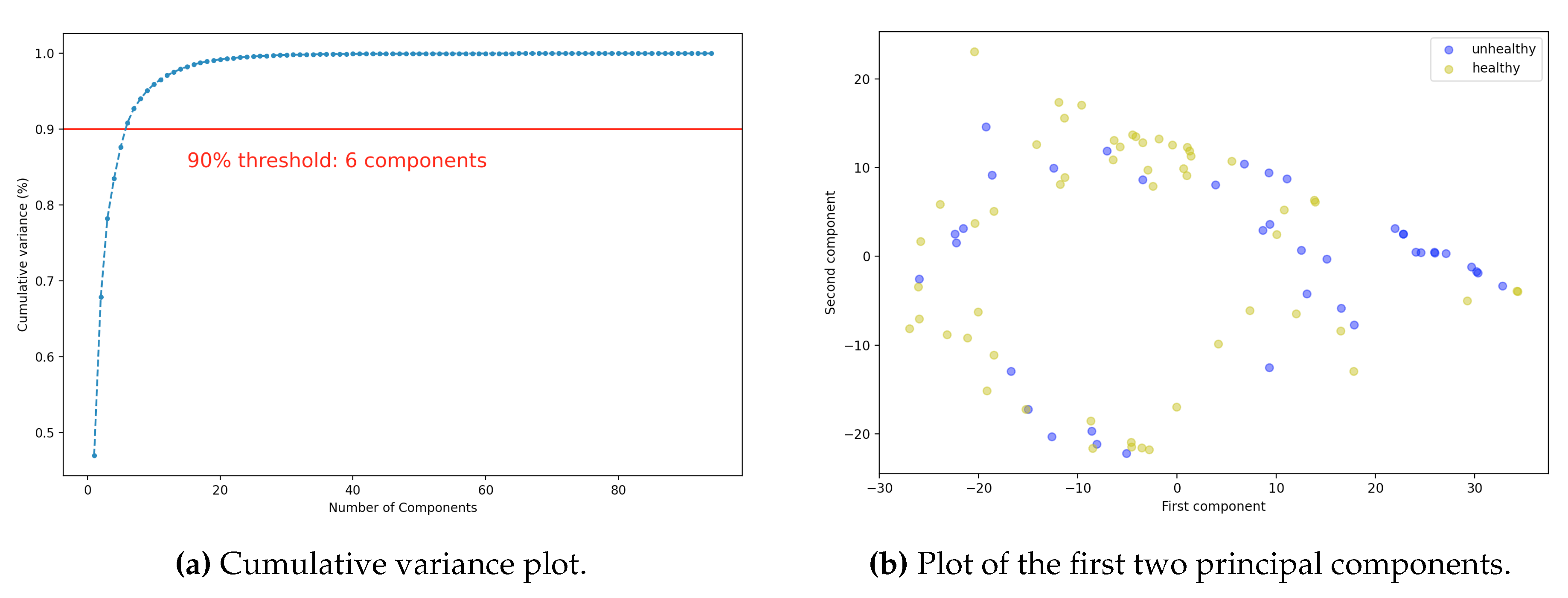
Concerning PCA, we selected 2 or 6 principal components. Considering the second case, more than 90% of the variance is captured, as shown in
Figure 5a. For ease of visualization, in
Figure 5b, the representation of the data with respect to the first two principal components is shown. As expected, the data distribution of healthy and diseased cells overlaps significantly.
2.3.3. SVM classifiers
Once the AEs’ outputs have been concatenated, or after PCA, the compressed spectra are presented to an SVM classifier. Three types of kernels have been tested: linear, polynomial and RBF, whose parameters were selected based on a grid search. Moreover, in the case of the 1D–CAEs, before classification, the channels of the compressed spectra must be concatenated, so that single vectors are fed into the classifier.
2.3.4. Evaluation metrics
The quality of compressed data has been evaluated using three common metrics [
32], namely Compression Ratio (CR), Root Mean Squared Error (RMSE) and Percentage Root mean squared Difference (PRD).
In particular, CR is the ratio between uncompressed and compressed data size:
where
N is the length of uncompressed data and
M is the dimension of the compressed patterns. This ratio estimates the compression efficiency — higher CR means higher compression — so it is desirable to be as high as possible.
RMSE is widely used to estimate the variance between reconstructed and original signals:
where
and
are the original and reconstructed signal, respectively. RMSE is a measure of the loss of information due to the compression. While lossless compression algorithms should ideally ensure fully informative compressed data, some small loss can still occur due to quantization errors.
Finally, PRD is given by:
which is a measure of the percentage of information loss.
On the other hand, classification performance has been evaluated based on accuracy, precision, and recall, defined as:
where
,
,
and
represent the true positive, true negative, false positive, and false negative predicted values, respectively.
3. Experimental results
In this section we present the comparative performance of different AE–based models, in order to select the most accurate architecture to compress NMR spectra. As a subsequent verification of the quality of the compression procedure, the compressed spectra were then classified as descriptive of healthy or diseased cells.
Table 2 summarizes the compression performance of all the tested autoencoders. In the table, the model name explains the AE structure, e.g.,
704_emb 2_lay means that the MLP–AE has two layers for both the encoder and the decoder while the whole latent space has dimension 704 (with 16 neurons for each compressed sub–spectrum embedding). Concerning 1D–CAEs,
4_ch means that the compressed spectrum has 4 channels to be concatenated to evaluate the embedding length, while
3_lay is the number of the encoder layers. Using 3 layers with stride 5 reduces the data dimensionality by a factor of
, producing a compressed sub–spectrum with dimension
, and a complete compressed spectrum described by a vector consisting of
entries. Finally, the decoder has one more 1D convolutional layer to produce an output with the same dimension of the input.
As can be seen from
Table 2, the reconstruction error is always small, while the PRD maintains under 1%; moreover, for comparable compression efficiency values (CR column), the best RMSE and PRD come from the 1D–CAE models. Actually, the CR metrics is always very high, reaching the maximum value of 312.5 for the 1D–CAE with 4 channels and 5 layers (embedding dimension equal to 176) and for the MLP–AEs with both 2 and 3 layers and 16 neurons in the last layer (embedding dimension equal to 704). However, the minimum for RMSE and PRD is obtained with the 1D–CAE with 8 channels and 3 layers (RMSE
and PRD
), where the value of CR is comparatively small (in line with our expectations).
The classification task has been carried out by a SVM with a RBF kernel, which was chosen after testing also linear and polynomial kernels. A grid search approach was used in order to find the best kernel parameters (
and
). For performance evaluations, due to the very small number of available examples, a leave–one–out technique was implemented. Each experiment consists of 94 training/test runs, each of which reserves a single pattern for testing, while the other 93 are used in the training phase. The held–out test example is different at every run. The results obtained for each AE model are synthesized also in
Table 2.
The accuracy of all models is about 76% and reaches its maximum value for the MLP–AE with 2 layers and embedding dimension equal to 2816, and for the 1D–CAE with 4 channels and 4 layers (embedding dimension equal to 1408), where it exceeds 77%. For these two models, the precision remains the highest (respectively 73% and 73.6%), while the recall never falls below 96% (respectively 98.2% and 96.4%). These results — which surpass those obtained with the PCA calculated on the original NMR spectra — indicate that the AE–based compression allows the extraction of features of better quality, which can be efficiently used for classification, (see
Table 3). Indeed, while the 6D–PCA maintains slightly lower accuracy values, this cannot be said for the 2D–PCA, with which about 7% of accuracy is lost. Concerning the two best AE–based models, the 1D–CAE is absolutely preferable due to the significantly lower number of parameters (
against
) and because of its shorter embedding length (
against
components).
Finally, let us notice that, based on the values of both precision and recall, the classifier shows better performance in the recognition of healthy cells (positive patterns), with a recall grater than 0.94 for all models. This is not astonishing since the dataset is imbalanced, with the positive class containing around 60% of available data. Indeed, for imbalanced classification problems, the majority class is typically referred to as the negative outcome and the minority class is typically referred to as the positive outcome. Actually, the precision calculated on the diseased class for the 1D–CAE architecture of
Table 3 is equal to 0.91, assessing that the patterns which the classifier recognizes as belonging to this class are almost always spectra of diseased cells.
4. Conclusion
In vitro cell–based metabolomics studies, often combined with other –omics, have found widespread use in many research areas, including analysis of drug effect, action, and toxicology, tumor cell characterization and signature extraction from cells. Indeed, cell signatures can constitute biomarkers usable for the early diagnosis of widespread pathologies, like Alzheimer’s Disease. In fact, the common goal of metabolomics studies is to understand and decipher the influence and involvement of metabolism in biological effects and mechanisms, and integrate this information onto metabolic maps. However, analyzing the metabolic phenotype of cells using NMR spectroscopy and artificial intelligence tools is a branch of research still in its embryonic phase. In this paper, we have proposed a whole pipeline to process NMR spectra in order to automatically establish if they correspond to a signature of a healthy or diseased cell. Identification of metabolite biomarkers depends on determining the latent variables responsible for class separation (healthy vs. diseased). PCA identifies the largest variations in the NMR data, but the latent variables responsible for class separation may not be in the direction of the largest variation. Instead, based on DL techniques, we have proved that high–dimensional NMR data can be embedded in compact representations — in ad hoc latent spaces —, which can be used to represent the spectra in an information–conservative way, usable for automatic classification. Preliminary but promising results show the ability of the proposed method to distinguish between healthy and diseased neuronal cells, for the early diagnosis of neuro–degenerative pathologies. The significantly reduced dimension of embedded spectra, obtained with almost no information loss, would allow to drastically reduce both the computational cost and memory storage, opening the door to the intensive use of automatic processing techniques for NMR data (not only related to the metabolic cell profile).
Author Contributions
Conceptualization, M.B. and F.C.; methodology, F.C., A.K, D.V., F.S. and M.B.; software, F.C.; validation, M.B. and F.C.; formal analysis, F.C.; investigation, F.C. and A.K.; resources, F.C., D.V. and A.K.; data curation, D.V. and A.K.; writing—original draft preparation, F.C. and A.K.; writing—review and editing, M.B. and D.V.; visualization, F.C. and A.K.; supervision, M.B., D.V. and F.S.; project administration, F.C., A.K., D.V., F.S. and M.B.; funding acquisition, D.V. All authors have read and agreed to the published version of the manuscript.
Funding
This research received no external funding.
Institutional Review Board Statement
Not applicable.
Acknowledgments
Consorzio Interuniversitario Risonanze Magnetiche di Metallo Proteine (CIRMMP) is acknowledged for scholarship support. Paolo Andreini is acknowledged for helpful discussion on CNNs and autoencoders.
Conflicts of Interest
The authors declare no conflict of interest.
Abbreviations
The following abbreviations are used in this manuscript:
| AD |
Alzheimer’s Disease |
| AE |
AutoEncoder |
| ATM |
Automatic Tuning–Matching |
| CAE |
Convolutional AutoEncoder |
| CR |
Compression Ratio |
| DL |
Deep Learning |
| ECG |
ElectroCardioGram |
| LDA |
Linear Discriminant Analysis |
| MLP |
MultyLayer Perceptron |
| MLP–AE |
MultyLayer Perceptron AutoEncoder |
| ND |
Neurodegenerative Disease |
| NMR |
Nuclear Magnetic Resonance |
| NOESY |
Nuclear Overhauser Enhancement SpectroscopY |
| NRU |
Neutral Red Uptake |
| PCA |
Principal Component Analysis |
| PRD |
Percentage Root–mean–square Difference |
| RBF |
Radial Basis Function |
| RMSE |
Root Mean Square Error |
| SVM |
Support Vector Machine |
| TMSP |
TriMethylSilylPropanoic acid |
| 1D–CAE |
1–Dimensional Convolutional Autoencoder |
|
nD–PCA |
n–Dimensional PCA |
References
- Kozlowski, H.; Luczkowski, M.; Remelli, M.; Valensin, D. Copper, zinc and iron in neurodegenerative diseases (Alzheimer’s, Parkinson’s and prion diseases). Coordination Chemistry Reviews 2012, 256, 2129–2141. [Google Scholar] [CrossRef]
- Stern, N.; et al. Dual Inhibitors of AChE and BACE–1 for Reducing Aβ in Alzheimer’s Disease: From In Silico to In Vivo. International Journal of Molecular Sciences 2022. [Google Scholar] [CrossRef]
- Nagu, P.; Pathan, A.K.A.; Mehta, V. Screening of Herbal Molecules for The Management of Alzheimer’s Disorder: In Silico and In Vitro Approaches. Applied Biological Research 2022, 24, 255–272. [Google Scholar] [CrossRef]
- Biedler, J.L.; Roffler-Tarlov, S.; Schachner, M.; Freedman, L.S. Multiple Neurotransmitter Synthesis by Human Neuroblastoma Cell Lines and Clones. Cancer research 1978, 11 Pt 1, 3751–3757. [Google Scholar]
- Luo, Y.; et al. Role of amber extract in protecting SH-SY5Y cells against amyloid beta 1-42-induced neurotoxicity. Biomedicine & Pharmacotherapy.
- Bell, M.; Zempel, H. A human cell model for TAU sorting and vulnerability. Reviews in the Neurosciences 2022, 33, 1–15. [Google Scholar] [CrossRef]
- Huang, K.; Thomas, N.; Gooley, P.R.; Armstrong, C.W. Systematic Review of NMR–Based Metabolomics Practices in Human Disease Research. Human Metabolites 2022. [Google Scholar] [CrossRef]
- da Silva, G.H.R.; Mendes, L.F.; de Carvalho, F.V.; de Paula, E.; Duarte, I.F. , Comparative Metabolomics Study of the Impact of Articaine and Lidocaine on the Metabolism of SH-SY5Y Neuronal Cells. Human Metabolites 2022. [Google Scholar] [CrossRef]
- Paris, D.; et al. Metabolic response of SH-SY5Y cells to gold nanoparticles by NMR–based metabolomics analyses. Human Metabolites 2016. [Google Scholar] [CrossRef]
- Corsaro, C.; Vasi, S.; Neri, F.; Mezzasalma, A.M.; Neri, G.; Fazio, E. NMR in Metabolomics: From Conventional Statistics to Machine Learning and Neural Network Approaches. Applied Sciences 2022, 12, 2824. [Google Scholar] [CrossRef]
- Klukowski, P.; Riek, R.; Güntert, P. , Rapid protein assignments and structures from raw NMR spectra with the deep learning technique ARTINA. Nature Communications 2022, 13, 1–12. [Google Scholar] [CrossRef] [PubMed]
- Klukowski, P.; Augoff, M.; Zięba, M.; Drwal, M.; Gonczarek, A.; Walczak, M.J. , NMRNet: a deep learning approach to automated peak picking of protein NMR spectra. Bioinformatics 2018, 34, 2590–2597. [Google Scholar] [CrossRef] [PubMed]
- Luo, J.; Zeng, Q.; Wu, K.; Lin, Y. , Fast reconstruction of non–uniform sampling multidimensional NMR spectroscopy via a deep neural network. Journal of Magnetic Resonance, 2020, 317, 106772. [Google Scholar] [CrossRef]
- Jo, T.; Nho, K.; Saykin, A.J. Deep Learning in Alzheimer’s Disease: Diagnostic Classification and Prognostic Prediction Using Neuroimaging Data. Frontiers in Aging Neuroscience 2019, 11. [Google Scholar] [CrossRef] [PubMed]
- Liu, S.; Masurkar, A.V.; Rusinek, H.; et al. Generalizable deep learning model for early Alzheimer’s disease detection from structural MRIs. Scientific Reports 2022, 12, 17106. [Google Scholar] [CrossRef] [PubMed]
- Rossi, A.; Vannuccini, G.; Andreini, P.; Bonechi, S.; Giacomini, G.; Scarselli, F.; Bianchini, M. Analysis of brain NMR images for age estimation with deep learning. Procedia Computer Science 2019, 159, 981–989. [Google Scholar] [CrossRef]
- Qiu, S.; Miller, M.I.; Joshi, P.S.; et al. Multimodal deep learning for Alzheimer’s disease dementia assessment. Nature Communications 2022, 13, 3404. [Google Scholar] [CrossRef]
- Wisely, C.E.; Wang, D.; Henao, R.; et al. Convolutional neural network to identify symptomatic Alzheimer’s disease using multimodal retinal imaging. British Journal of Ophthalmology 2022, 106, 388–395. [Google Scholar] [CrossRef]
- Cheung, C.Y.; et al. A deep learning model for detection of Alzheimer’s disease based on retinal photographs: a retrospective, multicentre case–control study. The Lancet — Digital Health 2022, 4, E806–E815. [Google Scholar] [CrossRef]
- Kola, A.; Lamponi, S.; Currò, F.; Valensin, D. A Comparative Study between Lycorine and Galantamine Abilities to Interact with AMYLOID β and Reduce In Vitro Neurotoxicity. International Journal of Molecular Sciences 2023, 24, 2500. [Google Scholar] [CrossRef]
- Cannella, V.; Altomare, R.; Leonardi, V.; Russotto, L.; Di Bella, S.; Mira, F.; Guercio, A. In vitro biocompatibility evaluation of nine dermal fillers on L929 cell line. BioMed Research International 2020. [Google Scholar] [CrossRef] [PubMed]
- Cannella, V.; Altomare, R.; Chiaramonte, G.; Di Bella, S.; Mira, F.; Russotto, L.; Pisano, P.; Guercio, A. Cytotoxicity Evaluation of Endodontic Pins on L929 Cell Line. BioMed Research International 2019, 2019, 3469525. [Google Scholar] [CrossRef] [PubMed]
- Rumelhart, D.E.; Hinton, G.E.; Williams, R.J. Learning internal representations by error propagation. In Parallel distributed processing: explorations in the microstructure of cognition, vol. 1: foundations; MIT Press; Publishing House: Cambridge, MA, USA, 1986; pp. 318–362. [Google Scholar]
- Bank, D.; Koenigstein, N.; Giryes, R. Autoencoders, 2020. [CrossRef]
- Ryu, S.; Choi, H.; Lee, H.; Kim, H. Convolutional Autoencoder Based Feature Extraction and Clustering for Customer Load Analysis. IEEE Transactions on Power Systems 2020, 35, 1048–1060. [Google Scholar] [CrossRef]
- An, J.; Cho, S. Variational autoencoder based anomaly detection using reconstruction probability. Special Lecture on IE 2015, 1–18. [Google Scholar]
- Gong, D.; Liu, L.; Le, V.; Saha, B.; Mansour, M.R.; Venkatesh, S.; Hengel, A.V.D. Memorizing normality to detect anomaly: Memory–augmented deep autoencoder for unsupervised anomaly detection. In Proceedings of the IEEE/CVF International Conference on Computer Vision 2015; 1705–1714. [Google Scholar]
- Xu, W.; Keshmiri, S.; Wang, G. Adversarially approximated autoencoder for image generation and manipulation. IEEE Transactions on Multimedia 2019, 21, 2387–2396. [Google Scholar] [CrossRef]
- Semeniuta, S.; Severyn, A.; Barth, E. A hybrid convolutional variational autoencoder for text generation. arXiv, arXiv:1702.02390.
- Wan, Z.; Zhang, Y.; He, H. Variational autoencoder based synthetic data generation for imbalanced learning. IEEE Symposium Series on Computational Intelligence (SSCI) 2017, 1–7. [Google Scholar]
- Wang, F.; Ma, Q.; Liu, W.; Chang, S.; Wang, H.; He, J.; Huang, Q. A novel ECG signal compression method using spindle convolutional auto–encoder. Computer Methods and Programs in Biomedicine 2019, 175. [Google Scholar] [CrossRef]
- Tiwari, A.; Falk, T.H. Lossless electrocardiogram signal compression: A review of existing methods. Biomedical Signal Processing and Control 2019, 51, 338–346. [Google Scholar] [CrossRef]
|
Disclaimer/Publisher’s Note: The statements, opinions and data contained in all publications are solely those of the individual author(s) and contributor(s) and not of MDPI and/or the editor(s). MDPI and/or the editor(s) disclaim responsibility for any injury to people or property resulting from any ideas, methods, instructions or products referred to in the content. |
© 2023 by the authors. Licensee MDPI, Basel, Switzerland. This article is an open access article distributed under the terms and conditions of the Creative Commons Attribution (CC BY) license (http://creativecommons.org/licenses/by/4.0/).
