
Submitted:
28 April 2023
Posted:
29 April 2023
You are already at the latest version
Abstract
In the era of big data, feature engineering has proved its efficiency and importance in dimensionality reduction and useful information extraction from original features. Feature engineering can be expressed as dimensionality reduction and is divided into two types of methods such as feature selection and feature extraction. Each method has its pros and cons. There are a lot of studies to combine these methods. Sparse autoencoder (SAE) is a representative deep feature learning method that combines feature selection with feature extraction. However, existing SAEs do not consider the feature importance during training. It causes extracting irrelevant information. In this paper, we propose a parallel guiding sparse autoencoder (PGSAE) to guide the information by two parallel guiding layers and sparsity constraints. The parallel guiding layers keep the main distribution using Wasserstein distance which is a metric of distribution difference, and it suppresses the leverage of guiding features to prevent overfitting. We perform our experiments using four datasets that have different dimensionality and number of samples. The proposed PGSAE method produces a better classification performance compared to other dimensionality reduction methods.
Keywords:
dimensionality reduction
; autoencoder
; feature extraction
; feature selection
; guiding layer
; regularization
1. Introduction
Efficient feature learning algorithms have become an essential element and the hot research topic in the era of big data [1]. Massive and high-dimensional data has generally a lot of redundancies and noise. It brings us huge challenges to extract important features, process them, and identify meaningful pattern. Many traditional methods are also fine in some cases. For example, many methods are based on linear relationships. It is intuitive and easily understandable. However, there are also non-linear data structures. Therefore, the machine learning-based model can be a solution to explain the non-linear structure. Autoencoder [2,3,4,5] is a representative machine learning technique for finding manifolds that represent large-scale data and is employed vastly in the field of feature extraction and dimensionality reduction. It consists of two parts: an encoder and a decoder. The encoder transforms the input into a latent vector that contains the main information. The decoder reconstructs the latent vector to new features same as the input form. It learns to minimize the reconstruction error. This method has become one of the useful feature engineering methods.
Feature engineering is a process of extracting important information from raw data and can be generally divided into two types: feature selection [6,7,8] and feature extraction [9,10]. Feature selection can be explained as a method of finding a subset of features with higher feature importance for classification. Therefore, it is possible to effectively remove less relevant features. These methods generally have a high generalization performance and computational efficiency. For example, there is a regularization [11,12], information gain [13], chi-square test [14], etc. However, this method has the disadvantage of removing potential non-noise factors of the original data. On the other hand, feature extraction methods are usually based on the reconstruction of features and projection from high-dimensional data into low-dimensional subspace. This kind of algorithm normally preserves the variance of features, so it has high information retention. However, since these algorithms consider almost all features in the transformation process, the dimensionality reduction effect is usually depleted. Principal component analysis (PCA) [15,16], canonical correlation analysis (CCA) [17], linear discriminant analysis (LDA) [18,19], and autoencoder using machine learning models for feature extraction are representative methods.
However, autoencoder has overfitting problems and highly complex structural issues. Improved structures have been proposed in recent years to solve these problems. Peicheng et al. [20] applied a stacked autoencoder (SAE) to hyperspectral image classification to generate high-quality hyperspectral image data to maximize the performance of the task. Meidi et al. [21] applied a stacked autoencoder to fault diagnosis of rolling bearings and obtained promising results. They increase the size of the network to get a better result. However, the autoencoder-based simple method is still a field of feature extraction, so it is difficult to modify and remove features with less relevance, which is the advantage of feature selection. To improve this shortcoming, new techniques applying regularization have been studied. Especially, stacked sparse autoencoder [22,23,24] is one of the representative deep autoencoder methods which have feature selection ideas. Stacked sparse autoencoder (SSAE) improved the autoencoder by a combination of two advanced autoencoders: a sparse autoencoder and stacked autoencoder. A sparse autoencoder adds sparse constraints to the autoencoder. It restricts the useless node to reduce the dimension efficiently. A stacked autoencoder improves the training performance by stacking autoencoders. It mediates to deeply learn the features in comparison to the simple learning process of traditional autoencoders. Anush et al. [25] proposed the structure of group sparse autoencoder (GAE) with regularization applied to solve the overfitting, which is a chronic problem of autoencoders.
Although SSAE’s regularization-based methods achieved successful results in various applications, due to its structural issues, it is difficult to apply the dynamic and efficient feature selection method. In many cases, there are vanishing gradient problems and over-generalizing information (e.g., on sensitive applications). Zhilei et al. [26] proposed a label and sparse regularization autoencoder (LSRAE). The main idea of LSRAE is to learn by dividing the output layer of the autoencoder into two parts, the actual label and output data, to extract features that involve the relationship between features and targets, and to prevent overfitting via sparse regularization. Most of the regularization-based autoencoders optimize the loss function without considering the structure. However, LSRAE has structural changes and the advantages of supervised learning. This is an important point in the feature engineering field. Hongteng et al. [27] proposed a relational regularized autoencoder (RAE) that flexibly learns a structured prior distribution using Fused Gromov-Wasserstein (FGW) [28] distance. The main idea is to limit the difference by regularizing the structural distance between the latent prior and the corresponding posterior using a metric that determines the distribution similarity. Therefore, to obtain high-quality and low-dimensional features, the structure of SSAE needs to be improved and reformed.
In this paper, we propose a parallel guiding sparse autoencoder (PGSAE) which is a deep advanced autoencoder model. PGSAE is a solution to the above-mentioned problems. The proposed PGSAE focuses on two parts: advanced structure and regularization. It is a structure that can effectively utilize feature importance analysis, which is the advantage of feature selection, in the autoencoder. There are two guiding layers before and after the reconstruction layer (output layer of the autoencoder) to adjust the leverage of feature importance. Guiding layers are for regularization of the autoencoder and limit their distributive difference by using Wasserstein distance to improve the performance of regularization. Therefore, it is a new manifold learning method that can improve the quality of deep features and obtain low-dimensional features.
Main Contributions
The main contributions of our method are summarized as follows:
- We introduce a new regularization method to apply flexible interaction of features on autoencoder. Unlike current autoencoder-based regularization methods which just deactivate the node of low activation probability, two guiding layers of our PGSAE method are complementarily trained to reduce the noise using the results of reconstruction.
- We propose a method based on Wasserstein distance. Wasserstein limits the relative distance of two guiding layers to improve the regularization performance. This offers a highly flexible regularization because it tunes the distributions of two guiding layers as a proper similarity and thus reduces information loss. Therefore, it can be a supplementary solution to the autoencoder-based feature learning method.
- We design a parallel network form. The parallel guiding process is quite a new concept. It can be extended to many neural network fields, where two different networks can be reasonably fused in terms of the probabilistic distribution.
- We develop the partially focused learning method by guiding the layer. It is the basic study to be applied to any other kind of neural network field and extended to be used in complex structures.
- The rest of this paper is organized as follows. Section 2 introduces the related work, including the basic theory and advanced theory of the autoencoder which is related to the proposed method. Section 3 describes the details of the proposed PGSAE method and shows its framework. Section 4 illustrates the experiment environment, evaluation metrics, information on datasets, and experimental results. Finally, Section 5 concludes the paper.
2. Background and Related works
In this section, we describe the autoencoder based models.
2.1. Sparse Autoencoder (SAE)
An autoencoder consists of two parts: an encoder and a decoder. In the encoder step, autoencoder transforms the original feature into latent representation. It is model-interpretable information. In the decoder step, autoencoder reconstructs the latent representation into new meaningful features.
An encoding function maps the input data sample to a low-dimensional latent feature space . It is formulated as:
where is the weight matrix between the input layer and hidden layer, is the activation function, is a bias and is a latent vector of the hidden layer. A decoding function maps to reconstructed feature . It can be expressed as:
where is the weight matrix between the hidden layer and output layer. The purpose of the autoencoder is to find a structure that minimizes the reconstruction error, and the objective function is defined as follows:
where is a amount of input samples. SAE’s structure is based on autoencoder. However, in basic autoencoder, when reconstructing input, the distribution of reconstructed features has a lot of overlap due to problems such as overfitting [29] and simply copy input and may not represent key information well. To solve these problems, we add a sparsity constraint as a penalty term that can suppress the output of neurons when the number of neurons in the hidden layer is large and formulated as follows:
where is the activation probability, is the sparse parameter. KL divergence is briefly a measure of how differences between two probability distributions [30].
2.2. Label and sparse regularization autoencoder (LSRAE)
Zhilei et al. proposed LSRAE, a structure that combines supervised learning methods with the autoencoder, which is unsupervised learning, to improve the performance of classification tasks. They thought that the overfitting and the irregular information problem of classification, which are chronic problems of autoencoders, occur because the relation between the target data and the input data is not considered at all in the reconstruction process. Therefore, they solved the problem by introducing the two main methods: First is adding a label regularization term to the objective function to reduce the difference between the actual label and the desired label and second is using the extreme learning machine [31] for fast optimization. LSRAE with label regularization term added is based on sparse autoencoder and formulated as follows:
where is the actual label as the output of autoencoder, is the desired label and is the number of input samples. Figure 1 shows a way to utilize the extreme learning machine (ELM) on autoencoder. Blue lines and red lines connect the hidden layer and the output layer and the label layer, respectively. ELM is utilized to obtain the output layer. It improves the classification accuracies. And they also use the sparse constraint to restrict useless nodes. The simple objective function of LSRAE is calculated as follows:
where is the loss function of the basic autoencoder.
3. Parallel guiding sparse autoencoder
Autoencoder has traditionally been used as one of the dimensionality reduction methods such as PCA and LDA. However, when overfitting occurs in the learning process, the following two major problems occur. First, even if unrelated data is used as input, it transforms the data to similar distribution with a training set. Second, while learning the information of features with low importance, a noise can be recognized as important information which affects classification accuracy. To solve the problem, we propose a parallel guiding sparse autoencoder (PGSAE) that learns the manifold of selected features and guides it to the rest of the features.
As shown in Figure 2, PGSAE has a structure with two added guiding layers to the basic autoencoder so that the two layers are parallel. From left to right, it is composed in the order of input layer, hidden layer (with guiding layer), reconstruction layer, guiding layer (output layer). The whole process is explained in small five processes. In the first process of PGSAE, , are output of hidden units and output of first guiding units, respectively. The step to calculate and can be represented as follows:
where and are input data, is activation function, and are the weights and biases between the first and second layers, respectively. denotes a guided feature and denotes a guiding feature. The learning process of PGSAE can be divided into two parts: (a) to learn the guiding feature as a target from the guided feature to involve the relation between the two features, and (b) to reconstruct the guided feature. A pretrained model from guided feature to guiding feature is required to involve the relation between the features. The corresponding part of PGSAE maps the guided feature of the input layer to the guiding feature of the first guiding layer and is pretrained partially. The cost function of partial pretrained model is formulated as follows:
The cost function used for pretraining is also used as a regularization term for the objective function in Eq. (18).
In the second process, as the number of units in the hidden layer increases, there may be too much sparse information. As a sparse constraint, the average activity of the hidden unit is calculated. If it is an important unit, it is activated, and if not, it is deactivated. The sparsity criterion for determining the importance of a unit uses the Kullback-Leibler (KL) divergence. KL divergence is the relative entropy to measure the similarity between a sparsity parameter and the average activation probability . is the number of the hidden units. The average activation is represented as
And (KL divergence) is represented as
In the third process, there is a reconstruction loss and the loss can be calculated by the output vector of the reconstruction layer . The output of the reconstruction layer is calculated as follows:
where is activation function and and are the weights and biases between the hidden (first guiding) layer and reconstruction layers, respectively. The term is a typical loss used in the existing autoencoder and is the main loss of PGSAE. In general, the mean squared deviation is used for linear cases, and cross-entropy is used for non-linear cases. In this section, we compute using mean squared deviation. is computed as follows:
In the fourth process, PGSAE has a second guiding part. Its operation step is almost the same to get the first guiding layer and two guide layers operate complementarily. The second guiding regularization term is obtained by and calculated as follows:
The guiding term is computed by two guiding terms Eq. (3), (9), and formulated as follows:
According to the structure of Figure 2. described above, the objective function of PGSAE using the above three equations (5), (7), (10), and Wasserstein regularization term Eq. (12) is defined as:
where is the weight vector , three coefficients, and are to balance the , is the pretrained prior distribution which we assume it as real data distribution and is the latent variable distribution. The Wasserstein regularization term is explained in the next part and shown as:
where Eq. (12) is the lowest estimate of the expected value of among all joint probability distributions . However, the infimum in Eq. (12) is too intractable and complex. Kantorovich-Rubinstein duality suggests us the solution to replace the problem with a low complexity duality problem. It can be formulated as:
where means all ranges that satisfy 1-Lipschitz function and is a function about that satisfies 1-Lipschitz function. By adding a weight clipping parameter to the function to fit the duality condition, it can be expressed as follows:
PGSAE assumes that we already have good performance throught pretraining. Ultimately our remaining goal is to find the optimum to update , , through the Wasserstein regularization. That is, it should find optimal . Furthermore, we could consider and compute differentiating the changed through the back-propagation method in Eq. (14). via getting . According to the above methods, using back-propagation of the entire objective function is possible by gradient descent algorithm. In the partial derivative formula to optimize , bias is omitted to simplify the expression.
The weights is formulated in the order as follows:
Since is not affected by , when differentiation is performed, it is removed from and only remains. is computed as follows:
Since is the weight between the first guiding layer and the reconstruction layer, it is not affected by . Therefore, is removed. is computed as follows:
Since and must have the adjacent gradient value and are updated in parallel, the sum of partial derivatives with respect to and partial derivatives with respect to is used as gradients and updated simultaneously. is computed as follows:
Through the above methods, the main steps of PGSAE algorithm which is the guiding feature learning method are summarized as follows:
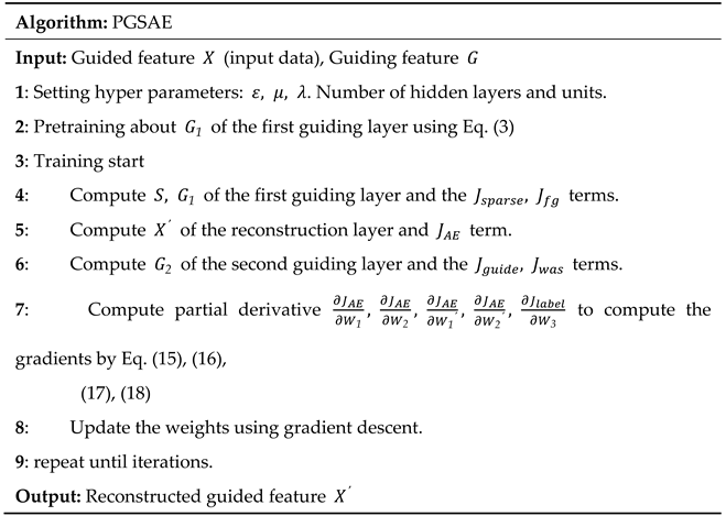 |
4. Experimental result of PGSAE
4.1. Datasets and experimental setups
In this paper, experiments are conducted using six public datasets with various dimensionality: Heart Disease (Heart) dataset, Wine quality (Wine) dataset, U.S. Postal Service (USPS) dataset, Fashion-MNIST dataset, Yale face (Yale) dataset and Columbia Object Image Library (COIL-100) dataset. The features of the dataset are divided into low-dimensional features, medium-dimensional features, and high-dimensional features. Brief information of the dataset is summarized in Table 1. We carry out the experiments on a personal server with the following configurations: two CPUs (AMD 7742 64-core), eight GPUs (NVIDIA DGX A100), memory (1 TB), and a NVMe Storage (15 TB).
The proposed PGSAE has three regularization terms: a parallel guiding term (), a sparse regularization term (), and Wasserstein regularization term ( in Eq. (18). The hyperparameters , and for the regularization term are defined, and we need to find the optimal coefficient suitable for different datasets. In particular, the parallel guiding coefficient and Wasserstein regularization parameter consider the leverage of the guiding feature. Thus, the classification performance depends on the sensitively tuned hyperparameters. The structure of PGSAE that contains guiding layers and the coefficients in this experiment are summarized in Table 2.
4.2. Authentication of main innovation
The main innovation of this study is to solve the overfitting problem of the autoencoder model, which is one of the dimensionality reduction algorithms, by applying a new regularization technique based on Wasserstein distance and guide layers. Overfitting of autoencoder is mainly divided into two categories: Learning the distribution of the identity function and transforming unrelated data like training data [32,33,34,35]. To solve these two overfitting categories, experiments were conducted in two phases. First, we designed an experiment to prove that PGSAE is not learning the distribution of identity functions. Second, the experiment was conducted to test whether the deep features extracted from PGSAE could potentially express main information rather than simply transforming the input data into the distribution of the training data to reduce the reconstruction error. In this section, an ablation study was applied to prove the performance of the basic structure of PGSAE and the effects of sparse regularizer and Wasserstein regularizer. Table 3 shows the results of using SVM as a classifier. The symbols in Table 3 are explained as follows. RF: raw features; DF: deep features trained by PGSAE without Wasserstein regularization and sparse regularization; DF & WR: deep features with Wasserstein regularization; DF & WR & SR: deep features with Wasserstein regularization and sparse regularization. As shown in Table 1 and Table 3, in most datasets, our methods have low-dimensional features compared to conventional RF, but the benchmark results show no significant performance degradation. DF & WR (DW) and DF & WR & SR (DWS) showed excellent results as follows: on the Heart, DWS shows 0.17% higher performance; on the Wine, DWS shows 0.59% lower performance; on the USPS, DW shows 1.42% lower performance; on the Fashion-MNIST, DWS shows 1.73% lower performance; on the Yale, DWS shows 3.21% lower performance; on the COIL-100, DWS shows 0.86% lower performance. In most cases, the performance slightly decreases, but the training efficiency increases a lot as follows: on the Heart, the efficiency increases about 31% from 13 features to 9; on the Wine, the efficiency increases about 33% from 12 to 8; on the USPS, the efficiency increases about 29% from 256 to 180; on the Fashion-MNIST, the efficiency increases about 29% from 784 to 549; on the Yale, the efficiency increases about 30% increase from 1024 to 717; on the COIL-100, the efficiency increases about 30% increase from 1024 to 717. Most of the results show a high learning efficiency of about 30%. Therefore, this strategy has been proven to be effective and can improve the performance and stability of the existing autoencoder model.
4.3. Comparison of the benchmark datasets
The efficiency of the proposed PGSAE is proven in Section 4.2, and in this section, we experiment to prove that PGSAE shows better performance than existing dimensionality reduction algorithms and does not learn the distribution of identity function. When the autoencoder model learns the distribution of the identity function to minimize the reconstruction error, it is difficult to expect improvement in classification because there are few transformations of the feature. Therefore, if the classification accuracy is improved compared to the result of using only the raw features by the hybrid feature of the deep features extracted from PGSAE and the raw features, it shows that our PGSAE is not overfitted without learning the distribution of the identity function. In Table 4, Hybrid PGSAE showed improvement in accuracy of 0.75%, 1.09%, 0.45%, 0.48%, 2.02%, and 0.57% for 6 datasets, respectively. This means that PGSAE does not learn the distribution of identity functions. In addition, Table 4 illustrates how much performance improvement of PGSAE was achieved compared to the existing feature extraction method through comparison experiments with representative dimensionality reduction algorithms. For comparison, the proposed PGSAE is compared with representative autoencoder models and dimensionality reduction methods as follows: Kernel PCA, LDA, stacked autoencoder (SAE), stacked sparse autoencoder (SSAE), uniform manifold approximation and projection (UMAP) and t-Stochastic neighbor embedding (t-SNE) [36,37,38]. As shown in Table 4, the proposed method in this study showed superior achievement in most cases compared to other methods on the six data sets. The PGSAE on the datasets Heart, USPS, Fashion-MNIST, and COIL-100 shows the best outcome compared to other dimensionality reduction techniques, and on the datasets Wine and Yale shows slightly lower performance at 0.62% and 0.13%, respectively, compared to the best algorithms. In addition, the accuracy of Hybrid PGSAE on the dataset Heart is 0.75% and 0.58% higher than that of RF and the best algorithm, respectively. In addition, the performance of Hybrid PGSAE on the Heart dataset is higher than RF and the best algorithm by 0.75% and 0.58%, respectively. Similarly, performance increase shows 1.09% and 1.06% on the Wine, 0.45% and 1.87% on the USPS, 0.48% and 2.21% on the Fashion-MNIST, 2.02% and 5.23% on the Yale, and 0.57% and 1.43% on the COIL-100, respectively to RF and the best algorithm. This means that the proposed method solved the overfitting issue of the autoencoder and displayed superior results.
4.4. Prevention of transforming irrelevant data as like training data
In Section 4.3, we proved that PGSAE does not learn the distribution of identity functions, but basically, the autoencoder performance relies on reconstruction quality, which is the most important component in the encoding-decoding process. The reconstruction error can still be an insufficient indicator due to other types of overfittings, and experiments to supplement are necessary. In this section, we compare the reconstruction error with the actual image simultaneously and show that the proposed PGSAE solves the overfitting that transforms the data unrelated to the training set into the distribution of the training set. In Figure 3, the experimental setup of the PGSAE on the datasets Fashion-MNIST and COIL-100 is illustrated in Table 2. In addition, Gaussian noise was used as an extra test set to confirm the transformation of the data distribution. In Figure 3, the PGSAE shows better restoration ability than the basic autoencoder model for detailed information. However, in Table 5, the reconstruction error of the PGSAE on the Fashion-MNIST and COIL-100 datasets is higher than the basic autoencoder. It means that the overfitting occurred because the basic autoencoder, which has lower reconstruction error, shows lower performance than the PGSAE. In Figure 3, the result of using Gaussian noise as an input value shows that most of the noise information is vaguely expressed in the case of a basic autoencoder. When there are many similar data in the training set, the reconstruction error can be reduced by transforming the information in this way, but the main information can be lost. PGSAE shows that this overfitting is improved through the guiding layer, Wasserstein regularization, and sparse regularization.
4.5. Effect of the coefficients and classifiers
4.5.1. Coefficients Optimization on the six datasets
In this experiment, two optimization techniques are used to find the optimum of the three coefficients and to be defined in PGSAE. The first one is a grid search algorithm that searches all values within a specific range and the second is a Bayesian optimization algorithm that probabilistically finds the optimal parameter composed of a surrogate model (Gaussian process) and an acquisition function [39,40,41]. Figure 4 shows the experimental results for coefficients and using grid search, and the ranges are and . Since is relatively more influential than and , we reduce the range of the sensitive coefficient by the results of grid search and additionally test the coefficient using Bayesian optimization algorithm to get a suitable value efficiently. The six datasets are split into two subsets: one accounting for about one-fifth of all samples as test data and the rest as the training data. We ran tests five times with randomly shuffled samples. As a classifier, SVM is chosen to optimize all coefficients. Figure 4 (a) shows the results of the parameter experiment on the Heart dataset. As the Wasserstein regularization parameter increases, the classification accuracy decreases. It shows superior outputs for values between about 0.003 and 0.004. The is the most important coefficient for extracting core features, and since the performance varies greatly depending on the data, the optimal value should be obtained through experiments. If it is too low, it causes a huge loss of the guiding feature and low accuracy of classification. Or if is too high, the weights are updated to improve the performance of guiding layers only. It brings a high reconstruction error of the PGSAE. The is the role to prevent overfitting. If is too low, the first guiding and second guiding layers are not interactive. In this case, the imbalanced guiding layers are updated only to reduce the reconstruction error thus overfitting occurs easily. If is too high, the first guiding layer and the second guiding layer become almost the same. It is too stiff to get optimal and leads to high reconstruction error. The is to filter sparse nodes out. It may increase or decrease the performance depending on the data and hidden unit. In Figure 4 (c), PGSAE showed better results when sparse regularization is not applied. Therefore, the parameter optimization process to get useful features is imperative in PGSAE. Figure 4 (b), (c), (d), (e), and (f) are the optimization result of Wine, USPS, Fashion-MNIST, Yale and COIL-100, respectively.
4.5.2. Effects of classifier
The classifier has a significant impact on the performance of PGSAE. We conducted an experiment using the following three representative classifiers: support vector machine (SVM), K-nearest neighbor (KNN), and random forest [42]. The experimental results are shown in Table 6. As a result, KNN shows poor performance in most cases in the proposed method. The random forest achieves higher accuracies than KNN in most cases and it is the highest accuracy on the Yale. However, in this experiment, it does not show optimal performance because all hyperparameters are set as default. Since SVM can be applied most stably to the proposed algorithm and shows excellent accuracies in most cases, it is chosen as a final classifier for PGSAE. Since the proposed PGSAE is in a field of dimensionality reduction and feature extraction domain, further experiments on different classifiers have not been carried out. However, if a more suitable and optimized classifier is used in the future work, performance can be improved, and it can be extended to other tasks.
5. Conclusion and future work
In this paper, we introduced a new method called PGSAE that works with parallel guiding layers. It is a dimensionality reduction method that combines the ideas of feature selection and feature extraction. There are two key points. The first one is using guiding layers to flexibly update the weights. It offers the advantages of feature selection and manages the effects of each feature to reduce the classification performance loss. The second one is a constraint method by Wasserstein distance and KL divergence. Wasserstein distance prevents overfitting in guiding layers and KL divergence restricts the useless nodes of the network. These two main ideas interactively perform to extract the main information of the origin feature and reduce the dimensionality. In the experiment, we compared PGSAE with other traditional dimensionality reduction methods and showed the performance differences according to classifiers on the Pima, heart, wine, and musk datasets. The proposed method outperforms other methods on average and shows the highest classification accuracies due to the coefficients of and are efficiently optimized through the experimental tests.
Feature work includes improving PGSAE in two ways. The first is through optimization methods. PGSAE is a sensitive model. Therefore, the optimization process is necessary. Thus, the next step is to generalize this model to utilize in other applications. The second one is by applying visualization using convolutional layers to ensure compatibility for image data and high dimensional data representation. Because dimensionality reduction methods are used not only for efficiency and performance but also for visualization to show a representative data structure.
Data Availability Statement
Every Dataset can be found as follows: Heart (https://archive.ics.uci.edu/ml/datasets/heart+disease), Wine (https://archive.ics.uci.edu/ml/datasets/wine+quality), USPS (https://www.csie.ntu.edu.tw/~cjlin/libsvmtools/datasets/multiclass.html#usps), Fashion-MNIST (https://www.kaggle.com/datasets/zalando-research/fashionmnist), Yale (http://vision.ucsd.edu/~leekc/ExtYaleDatabase/Yale%20Face%20Database.htm), COIL-100 (https://www.cs.columbia.edu/CAVE/software/softlib/coil-100.php).
Acknowledgments
This work was supported by Inha University Grant.
Conflicts of Interest
All authors declare that they have no conflicts of interest.
References
- D. Storcheus, A. Rostamizadeh, S. Kumar, A survey of modern questions and challenges in feature extraction, Feature Extraction: Modern Questions and Challenges, (PMLR2015), pp. 1-18.
- Wang, Y.; Yao, H.; Zhao, S. Auto-encoder based dimensionality reduction. Neurocomputing 2016, 184, 232–242. [Google Scholar] [CrossRef]
- Liou, C.-Y.; Cheng, W.-C.; Liou, J.-W.; Liou, D.-R. Autoencoder for words. Neurocomputing 2014, 139, 84–96. [Google Scholar] [CrossRef]
- Li, J.; Luong, M.-T.; Jurafsky, D. A hierarchical neural autoencoder for paragraphs and documents. arXiv preprint arXiv:1506.01057, 2015.
- Tschannen, M.; Bachem, O.; Lucic, M. Recent advances in autoencoder-based representation learning. arXiv preprint arXiv:1812.05069, 2018.
- Li, J.; Cheng, K.; Wang, S.; Morstatter, F.; Trevino, R.P.; Tang, J.; Liu, H. Feature selection: A data perspective. ACM Computing Surveys (CSUR) 2017, 50, 1–45. [Google Scholar] [CrossRef]
- Jović, A.; Brkić, K.; Bogunović, N. A review of feature selection methods with applications, 2015 38th international convention on information and communication technology, electronics and microelectronics (MIPRO), (Ieee2015), pp. 1200-1205.
- Chandrashekar, G.; Sahin, F. A survey on feature selection methods. Computers & Electrical Engineering 2014, 40, 16–28. [Google Scholar]
- Osia, S.A.; Taheri, A.; Shamsabadi, A.S.; Katevas, K.; Haddadi, H.; Rabiee, H.R. Deep private-feature extraction. IEEE Transactions on Knowledge and Data Engineering 2018, 32, 54–66. [Google Scholar] [CrossRef]
- Ghojogh, B.; Samad, M.N.; Mashhadi, S.A.; Kapoor, T.; Ali, W.; Karray, F.; Crowley, M. Feature selection and feature extraction in pattern analysis: A literature review. arXiv preprint 2019, arXiv:1905.02845. [Google Scholar]
- Schmidt, M.; Fung, G.; Rosales, R. Fast optimization methods for l1 regularization: A comparative study and two new approaches, European Conference on Machine Learning, (Springer2007), pp. 286-297.
- Van Laarhoven, T. L2 regularization versus batch and weight normalization. arXiv preprint 2017, arXiv:1706.05350. [Google Scholar]
- Azhagusundari, B.; Thanamani, A.S. Feature selection based on information gain. International Journal of Innovative Technology and Exploring Engineering (IJITEE) 2013, 2, 18–21. [Google Scholar]
- Bryant, F.B.; Satorra, A. Principles and practice of scaled difference chi-square testing. Structural equation modeling: A multidisciplinary journal 2012, 19, 372–398. [Google Scholar] [CrossRef]
- Mika, S.; Schölkopf, B.; Smola, A.J.; Müller, K.-R.; Scholz, M.; Rätsch, G. Kernel PCA and De-noising in feature spaces, NIPS1998), pp. 536-542.
- Ding, C.; Zhou, D.; He, X.; Zha, H. R 1-pca: rotational invariant l 1-norm principal component analysis for robust subspace factorization, Proceedings of the 23rd international conference on Machine learning2006), pp. 281-288.
- Andrew, G.; Arora, R.; Bilmes, J.; Livescu, K. Deep canonical correlation analysis, International conference on machine learning, (PMLR2013), pp. 1247-1255.
- Yu, H.; Yang, J. A direct LDA algorithm for high-dimensional data—with application to face recognition. Pattern recognition 2001, 34, 2067–2070. [Google Scholar] [CrossRef]
- Martinez, A.M.; Kak, A.C. Pca versus lda. IEEE transactions on pattern analysis and machine intelligence 2001, 23, 228–233. [Google Scholar] [CrossRef]
- Zhou, P.; Han, J.; Cheng, G.; Zhang, B. Learning compact and discriminative stacked autoencoder for hyperspectral image classification. IEEE Transactions on Geoscience and Remote Sensing 2019, 57, 4823–4833. [Google Scholar] [CrossRef]
- Sun, M.; Wang, H.; Liu, P.; Huang, S.; Fan, P. A sparse stacked denoising autoencoder with optimized transfer learning applied to the fault diagnosis of rolling bearings. Measurement 2019, 146, 305–314. [Google Scholar] [CrossRef]
- Coutinho, M.G.; Torquato, M.F.; Fernandes, M.A. Deep neural network hardware implementation based on stacked sparse autoencoder. IEEE Access 2019, 7, 40674–40694. [Google Scholar] [CrossRef]
- Shi, Y.; Lei, J.; Yin, Y.; Cao, K.; Li, Y.; Chang, C.-I. Discriminative feature learning with distance constrained stacked sparse autoencoder for hyperspectral target detection. IEEE Geoscience and Remote Sensing Letters 2019, 16, 1462–1466. [Google Scholar] [CrossRef]
- Xiao, Y.; Wu, J.; Lin, Z.; Zhao, X. A semi-supervised deep learning method based on stacked sparse auto-encoder for cancer prediction using RNA-seq data. Computer methods and programs in biomedicine 2018, 166, 99–105. [Google Scholar] [CrossRef]
- Sankaran, A.; Vatsa, M.; Singh, R. A. Majumdar, Group sparse autoencoder. Image and Vision Computing 2017, 60, 64–74. [Google Scholar] [CrossRef]
- Chai, Z.; Song, W.; Wang, H.; Liu, F. A semi-supervised auto-encoder using label and sparse regularizations for classification. Applied Soft Computing 2019, 77, 205–217. [Google Scholar] [CrossRef]
- Xu, H.; Luo, D.; Henao, R.; Shah, S.; Carin, L. Learning autoencoders with relational regularization, International Conference on Machine Learning, (PMLR2020), pp. 1 0576–10586.
- Vayer, T.; Chapel, L.; Flamary, R.; Tavenard, R.; Courty, N. Fused Gromov-Wasserstein distance for structured objects. Algorithms 2020, 13, 212. [Google Scholar] [CrossRef]
- Liang, J.; Liu, R. Stacked denoising autoencoder and dropout together to prevent overfitting in deep neural network, 2015 8th international congress on image and signal processing (CISP), (IEEE2015), pp. 697-701.
- Goldberger, J.; Gordon, S.; Greenspan, H. An Efficient Image Similarity Measure Based on Approximations of KL-Divergence Between Two Gaussian Mixtures, ICCV2003), pp. 487-493.
- Huang, G.-B.; Zhu, Q.-Y.; Siew, C.-K. Extreme learning machine: a new learning scheme of feedforward neural networks, 2004 IEEE international joint conference on neural networks (IEEE Cat. No. 04CH37541), (Ieee2004), pp. 985-990.
- Steck, H. Autoencoders that don't overfit towards the Identity. Advances in Neural Information Processing Systems 2020, 33, 19598–19608. [Google Scholar]
- Probst, M.; Rothlauf, F. Harmless Overfitting: Using Denoising Autoencoders in Estimation of Distribution Algorithms. J. Mach. Learn. Res. 2020, 21, 78:71–78:31. [Google Scholar]
- Kunin, D.; Bloom, J.; Goeva, A.; Seed, C. Loss landscapes of regularized linear autoencoders, International Conference on Machine Learning, (PMLR2019), pp. 3560-3569.
- Pretorius, A.; Kroon, S.; Kamper, H. Learning dynamics of linear denoising autoencoders, International Conference on Machine Learning, (PMLR2018), pp. 4141-4150.
- Bunte, K.; Haase, S.; Biehl, M.; Villmann, T. Stochastic neighbor embedding (SNE) for dimension reduction and visualization using arbitrary divergences. Neurocomputing 2012, 90, 23–45. [Google Scholar] [CrossRef]
- McInnes, L.; Healy, J.; Melville, J. Umap: Uniform manifold approximation and projection for dimension reduction. arXiv preprint 2018, arXiv:1802.03426. [Google Scholar]
- McInnes, L.; Healy, J.; Melville, J. UMAP: uniform manifold approximation and projection for dimension reduction, (2020).
- Wang, H.; van Stein, B.; Emmerich, M.; Back, T. A new acquisition function for Bayesian optimization based on the moment-generating function, 2017 IEEE International Conference on Systems, Man, and Cybernetics (SMC), (IEEE2017), pp. 507-512.
- Snoek, J.; Larochelle, H.; Adams, R.P. Practical bayesian optimization of machine learning algorithms. Advances in neural information processing systems 2012, 25. [Google Scholar]
- Audet, C.; Denni, J.; Moore, D.; Booker, A.; Frank, P. A surrogate-model-based method for constrained optimization, 8th symposium on multidisciplinary analysis and optimization2000), pp. 4891.
- Lin, W.; Wu, Z.; Lin, L.; Wen, A.; Li, J. An ensemble random forest algorithm for insurance big data analysis. Ieee access 2017, 5, 16568–16575. [Google Scholar] [CrossRef]
Figure 1.
The virtual structure of autoencoder using ELM.
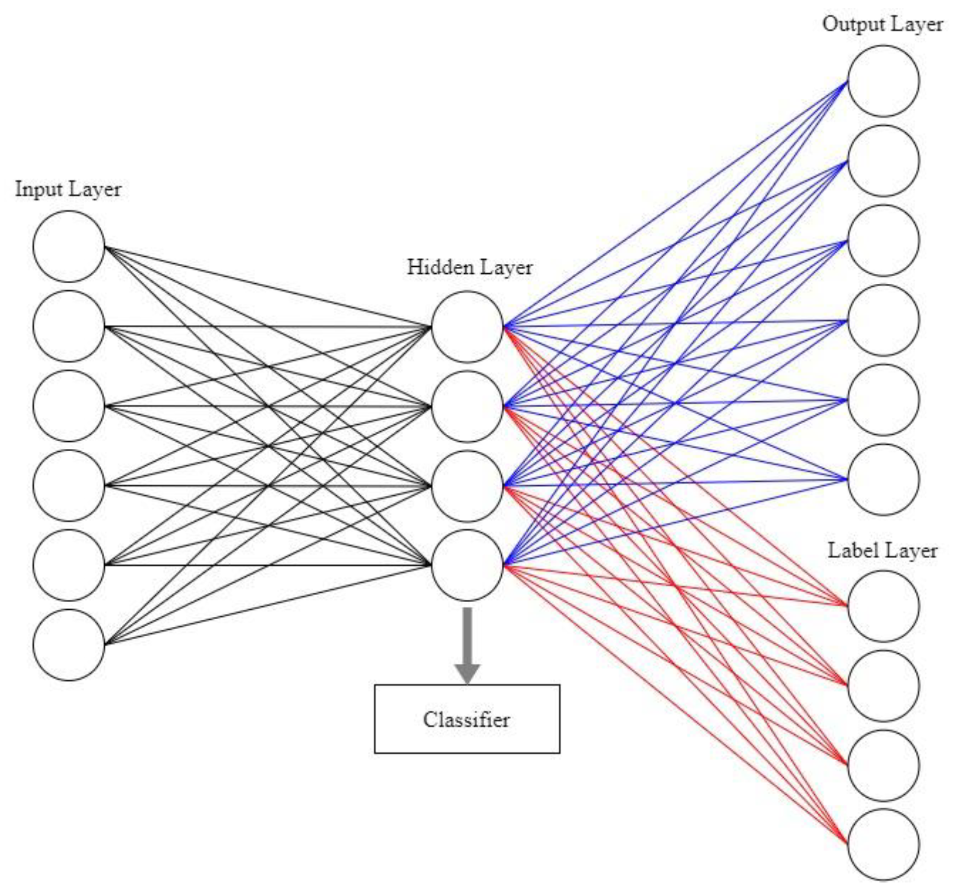
Figure 2.
The architecture of PGSAE. It consists of first guiding layer for the reconstruction of guided features and second guiding layer to reflect the distribution of guiding features.
Figure 2.
The architecture of PGSAE. It consists of first guiding layer for the reconstruction of guided features and second guiding layer to reflect the distribution of guiding features.
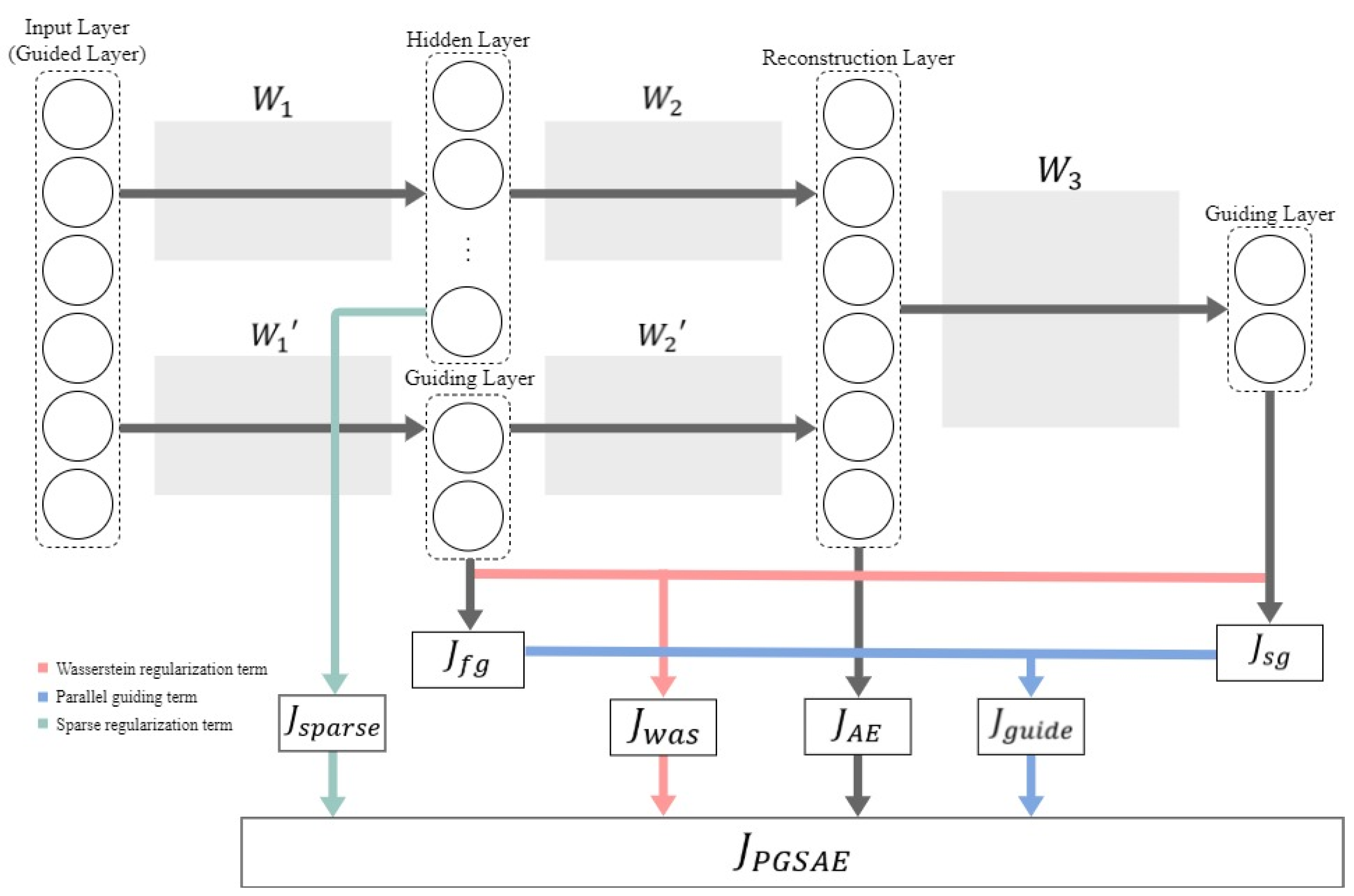
Figure 3.
Reconstructed image of Overfitted autoencoder model.
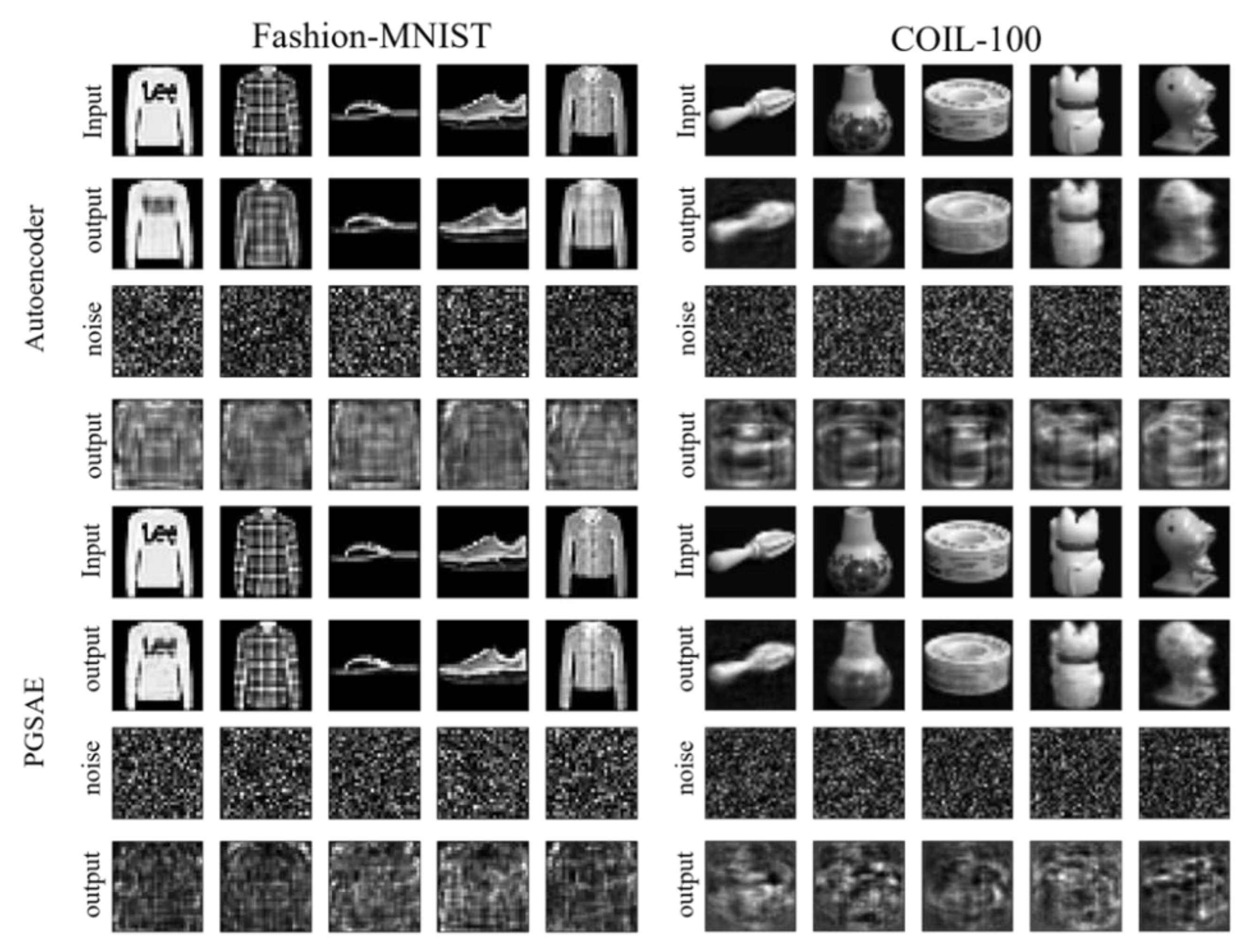
Figure 4.
Effects of the coefficients for classification accuracies on the six datasets: (a) Heart; (b) Wine; (c) USPS; (d) Fashion-MNIST; (e) Yale; (f) COIL-100;.
Figure 4.
Effects of the coefficients for classification accuracies on the six datasets: (a) Heart; (b) Wine; (c) USPS; (d) Fashion-MNIST; (e) Yale; (f) COIL-100;.
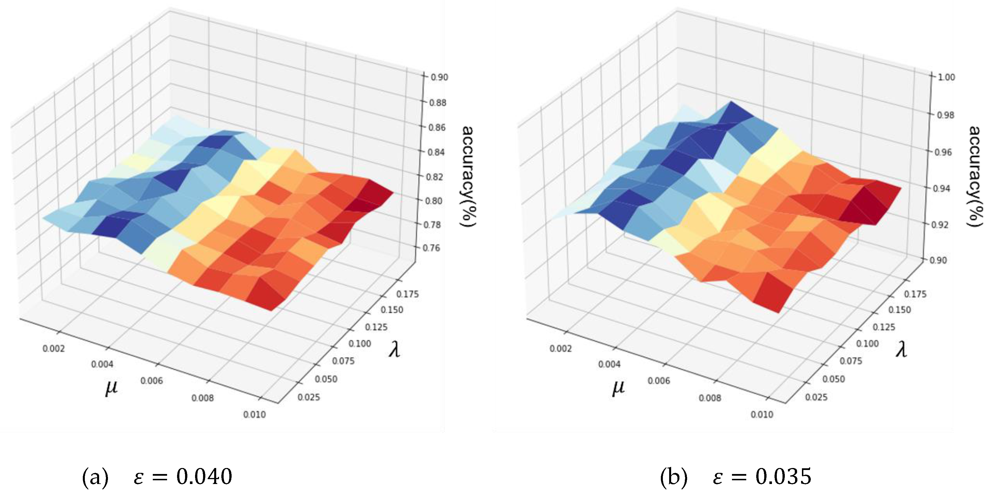
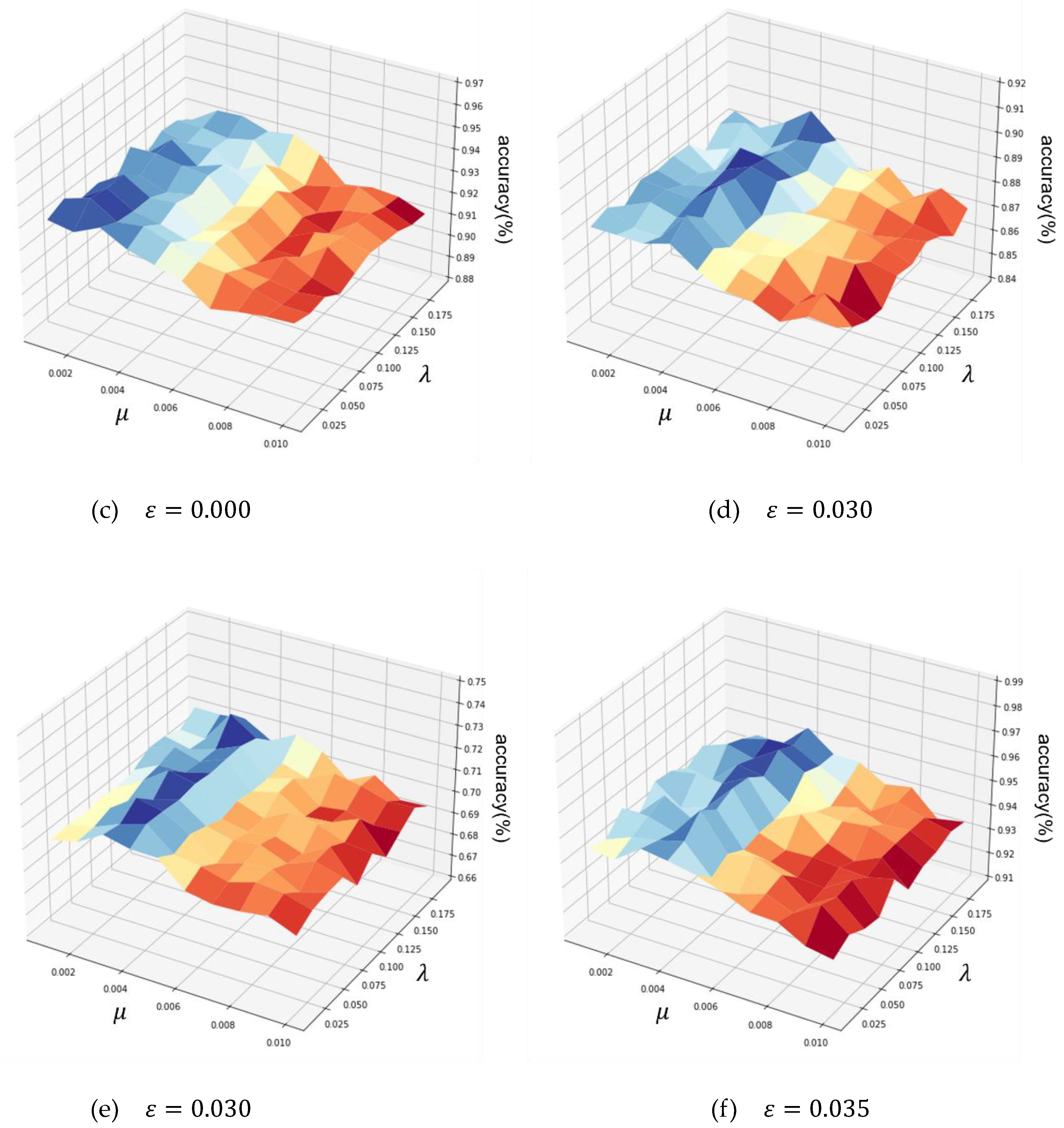

Table 1.
Summary of six public datasets.
| Dataset | # Classes | # Features | # Training | # Testing | # Dimensionality after feature extraction | |
| Low dimension | Heart | 2 | 13 | 240 | 63 | 9 |
| Wine | 2 | 12 | 4873 | 1624 | 8 | |
| Medium dimension | USPS | 10 | 256 | 7291 | 2007 | 180 |
| Fashion-MNIST | 10 | 784 | 60000 | 10000 | 549 | |
| High dimension | Yale | 15 | 1024 | 130 | 35 | 717 |
| COIL-100 | 100 | 1024 | 1080 | 360 | 717 | |
Table 2.
Parameters of PGSAE for six datasets.
| Dataset | # Guiding units of PGSAE | |||
|---|---|---|---|---|
| Heart | 64 – 32 – 64 | 0.040 | 0.119 | 0.004 |
| Wine | 64 – 32 – 64 | 0.035 | 0.166 | 0.003 |
| USPS | 256 – 128 – 256 | 0 | 0.025 | 0.001 |
| Fashion-MNIST | 256 – 128 – 256 | 0.030 | 0.115 | 0.003 |
| Yale | 512 – 256 – 512 | 0.030 | 0.171 | 0.002 |
| COIL-100 | 512 – 256 – 512 | 0.035 | 0.172 | 0.003 |
Table 3.
Ablation study on key components of PGSAE.
| Dataset | RF (%) | DF (%) | DF & WR (%) | DF & WR & SR (%) |
|---|---|---|---|---|
| Heart | 82.47 2.1 | 81.24 1.3 | 82.44 1.8 | 82.642.0 |
| Wine | 96.84 0.5 | 94.62 2.0 | 96.12 0.6 | 96.25 1.1 |
| USPS | 94.92 3.4 | 93.15 1.6 | 93.50 2.4 | 93.24 2.3 |
| Fashion-MNIST | 90.60 0.4 | 86.76 2.3 | 88.46 2.1 | 88.87 1.8 |
| Yale | 74.56 2.1 | 70.51 5.7 | 71.08 4.2 | 71.35 5.5 |
| COIL-100 | 96.19 0.2 | 93.87 1.1 | 94.56 1.2 | 95.33 0.5 |
Table 4.
Classification accuracies of three different classifiers by seven dimensionality reduction methods.
Table 4.
Classification accuracies of three different classifiers by seven dimensionality reduction methods.
| Dataset | RF (%) |
Kernel PCA (%) |
LDA (%) |
SAE (%) |
SSAE (%) |
UMAP (%) |
t-SNE (%) |
PGSAE (%) |
Hybrid PGSAE (%) |
| Heart | 82.47 2.1 |
81.82 1.1 |
76.86 4.5 |
82.23 2.8 |
81.82 2.7 |
74.38 5.2 |
60.33 9.2 |
82.64 2.0 |
83.22 1.7 |
| Wine | 96.84 0.5 |
96.00 1.2 |
93.15 1.4 |
95.98 1.5 |
96.87 1.1 |
95.54 2.2 |
95.52 2.9 |
96.25 1.1 |
97.93 0.8 |
| USPS | 94.92 3.4 |
91.46 5.6 |
92.78 5.7 |
93.47 3.9 |
93.23 4.5 |
89.23 9.9 |
86.36 8.4 |
93.50 2.4 |
95.37 3.1 |
| Fashion-MNIST | 90.60 0.4 |
87.07 3.5 |
87.27 3.2 |
87.98 2.7 |
88.65 1.8 |
81.28 6.4 |
81.38 4.7 |
88.87 1.8 |
91.08 1.0 |
| Yale | 74.56 2.1 |
71.48 6.8 |
68.26 3.6 |
67.44 7.4 |
70.78 4.1 |
69.33 5.5 |
61.45 8.5 |
71.35 5.5 |
76.58 4.2 |
| COIL-100 | 96.19 0.2 |
94.55 1.3 |
92.95 1.5 |
95.01 0.9 |
95.12 1.1 |
90.03 4.6 |
89.85 4.2 |
95.33 0.5 |
96.76 0.8 |
Table 5.
Reconstruction loss of the autoencoder models.
| Dataset | Basic AE (%) |
SAE (%) |
SSAE (%) |
PGSAE (%) |
|---|---|---|---|---|
| Heart | 0.3521 | 0.3213 | 0.3494 | 0.3132 |
| Wine | 0.4560 | 0.4651 | 0.4476 | 0.4242 |
| USPS | 0.1757 | 0.1634 | 0.1654 | 0.1537 |
| Fashion-MNIST | 0.2463 | 0.2578 | 0.2563 | 0.2487 |
| Yale | 0.8754 | 0.8743 | 0.8864 | 0.8435 |
| COIL-100 | 0.4749 | 0.4836 | 0.4798 | 0.4803 |
Table 6.
Classification accuracies of the PGSAE under different classifiers.
| Heart | Wine | USPS | Fashion-MNIST | Yale | COIL-100 | |
|---|---|---|---|---|---|---|
| SVM (%) | 82.64 2.0 | 96.25±1.1 | 93.50±2.4 | 88.87±1.8 | 71.35±5.5 | 95.33±0.5 |
| KNN (%) | 77.486.3 | 92.783.2 | 89.754.7 | 83.792.9 | 69.954.1 | 86.464.6 |
| Random Forest (%) | 81.721.8 | 94.552.1 | 90.562.2 | 86.782.7 | 72.174.8 | 94.811.4 |
Disclaimer/Publisher’s Note: The statements, opinions and data contained in all publications are solely those of the individual author(s) and contributor(s) and not of MDPI and/or the editor(s). MDPI and/or the editor(s) disclaim responsibility for any injury to people or property resulting from any ideas, methods, instructions or products referred to in the content. |
© 2023 by the authors. Licensee MDPI, Basel, Switzerland. This article is an open access article distributed under the terms and conditions of the Creative Commons Attribution (CC BY) license (http://creativecommons.org/licenses/by/4.0/).
Copyright: This open access article is published under a Creative Commons CC BY 4.0 license, which permit the free download, distribution, and reuse, provided that the author and preprint are cited in any reuse.


