Benveniste’s Experiments and the So-Called “Water Memory” Phenomenon: an Example of Serendipity? Investigation and Experiments

Francis BEAUVAIS

doi:10.20944/preprints202301.0155.v4

Preprint

Hypothesis

Benveniste’s Experiments and the So-Called “Water Memory” Phenomenon: an Example of Serendipity? Investigation and Experiments

This version is not peer-reviewed.

Francis BEAUVAIS^*

This version is not peer-reviewed.

Downloads

383

Views

253

Comments

Submitted:

06 May 2024

Posted:

10 May 2024

You are already at the latest version

Abstract

Benveniste’s experiments – known in the lay press as the “water memory” phenomenon – are generally considered to be a closed case. However, the amount of data generated by twenty years of well-conducted experiments prevents closing the file so simply. An issue, which has been little highlighted so far, merits to be emphasized. Indeed, if Benveniste failed to persuade his peers of the value of his experiments, it was mainly because of a stumbling block, namely the difficulty of convincingly proving the causal relationship between the supposed cause (“informed water”) and the experimental outcomes in different biological models. To progress in the understanding of this phenomenon, we abandon the idea of any role of water in these experiments (“water memory” and its avatars). In other words, we assume that “control” and “test” conditions to be evaluated were physically identical and differed only by their respective designations. We show in this article how simple probabilistic considerations allow to build a model that accounts for all aspects of Benveniste’s experiments. In this model based on probability amplitudes, constructive and destructive interferences emerge – or not – according to the experimental context. The recording of a statistical regularity shapes the intertwined whole constituted by the probability amplitudes of the states of the experimenter’s cognitive structures and of the experimental system. This model provides an alternative explanation to Benveniste’s experiments where water plays no role and where the place of the experimenter is central.

Keywords:

Water memory

;

High dilutions

;

Scientific controversy

;

Serendipity

;

Experimenter effect

Subject:

Medicine and Pharmacology - Other

1. Introduction

Serendipity has been defined as “the faculty or phenomenon of finding valuable or agreeable things not sought for” according to Merriam-Webster Dictionary [1]. This word was coined in 1754 by Horace Walpole as a reference to the fairy tale “The three princes of Serendip” from Cristoforo Armeno. The heroes of this story discovered by “chance and sagacity” things they were not looking for. The history of science is full of such chance discoveries as X-rays, radioactivity or penicillin. In this article, we will see why Benveniste’s experiments – also known in the lay press as the “water memory” phenomenon – could be a new example of serendipity.

The purpose of this article is not to tell again the entire story with all the details of the scientific debate and controversies that can be found elsewhere. A complete and systematic account of this case has been published by the author in a freely available text, both in a French version [2] and in its English translation [3]. Other points of views can be found in several books or articles [4,5,6,7,8,9,10,11,12]. The present article is hoped to be an element to reach a successful conclusion and, more importantly, to open new horizons.

It is important to remember that the experiments we are talking about were spread over almost 20 years (from 1983 to Benveniste’s death in 2003). This saga is too often reduced to the famous controversy with the journal Nature in 1988 [13,14]. Moreover, before this controversy, Benveniste had a position in the scientific community that was far from marginal. His research unit was affiliated with INSERM, the French national medical research institution, and Benveniste himself was recognized internationally. The original idea to test extreme dilutions was not from Benveniste himself who, as a good Cartesian, was rather reluctant initially to test homeopathic medicines, but was nevertheless open to countercurrent ideas. Indeed, homeopathy is an alternative medicine which, to put it mildly, is based on ideas from another time and has never proven its efficacy. B. Poitevin who was a thesis student at that time was also involved in the practice of homeopathy and proposed to Benveniste collaborations with the homeopathy industry [3,7]. Thus, the famous “Benveniste’s experiments” were initially nothing more than research contracts with homeopathy firms aimed to evaluate some homeopathic medications. It is important to notice that Benveniste’s team was not the first to test homeopathic medications. What was probably new was that a renowned laboratory from a public research institution managed such a research topic and that Benveniste did not hesitate to promote the high-dilution issue into the academic debate.

In the former experiments (years 1983–1991), high dilutions of various preparations were tested on human basophils which are cells involved in allergic disorders. Some of the diluted compounds were used in homeopathic practice, but others were not homeopathic medications (antibodies, for example). The hypothesis behind these first experiments performed in the 1980’ was that a drug or a biologically-active compound could apparently continue to manifest some activity after being highly diluted. Obtaining a specific effect on a biological model with high dilutions was theoretically impossible given physicochemical laws. To get an idea, less one molecule of antibody was theoretically present in the assay after about fifteen serial ten-fold dilutions of the initial sample. Therefore, the first positive results were received with surprise and skepticism in the laboratory, including Benveniste himself.

However, the basophil model needed fastidious and time-consuming counting under a microscope by trained experimenters and required a number of tricks to avoid pitfalls. In addition, the controversy with the journal Nature prompted Benveniste to consider other biological models. A physiological model already in use in the laboratory, namely the isolated rodent heart, appeared to be promising (years 1992–1998). Changes in the state of this biological model (coronary flow variations) could be followed live by observers and this new model was therefore more convincing and demonstrative than the basophil model. The results with high dilutions of various compounds were confirmed using the isolated rodent heart model [3].

After high dilutions, Benveniste developed from the year 1992 different devices based on electromagnetism and made of electric coils and electronic amplifiers which were supposed to “transfer the activity” of biologically-active molecules directly to water samples without the dilution process [3,15,16,17,18,19,20]. The “transmission” experiments were also supposed to avoid contaminations that could be responsible for the observed effects. In a further refinement, Benveniste obtained in 1995 experimental data suggesting that the “activity” issued from a biologically-active solution could be captured and stored in a computer memory. The electric current that passed through a coil surrounding a biologically-active sample was supposed to be modulated by an electromagnetic emission from the sample and was digitized before being stored in a computer file. Then the “biological activity” recorded in the file could be diffused via an electric coil to a water sample initially devoid of any “information”. In another variation of this device, the diffusion of the “biological activity” was done directly to the biological system via the electric coil without intermediate water sample. Benveniste coined at this occasion the term of “digital biology”. These new developments and his new ideas about a future breakthrough in biology and medicine thanks to “digital biology” further isolated Benveniste from the scientific community and caused him to lose his early supports.

The isolated heart rodent model, however, appeared to be difficult to export into other laboratories because few teams had the experience to use it routinely. Benveniste then developed experiments based on plasma coagulation that could be easily performed in most laboratories (years 1999–2001). This experimental model offered also the possibility of being completely automated. A robot that performed all steps of an experiment, including the random selection of experimental conditions and processing of biological samples, was thus developed. Again, the successful results obtained with this new device convinced Benveniste that he was on the right track. This robot attracted the attention of the US Defense Advanced Research Projects Agency (DARPA), which commissioned an expertise [21]. We will talk of the results of this expertise in the discussion section.

However, if these astonishing results were so obvious, why did Benveniste fail to convince his peers? The main reason was that he could not get rid of a strange phenomenon that literally poisoned his experiments, in particularly when he tried to carry out proof-of-concept experiments involving other researchers he wanted to convince. In Section 3, we will see what this stumbling block was and why it systematically and constantly stopped Benveniste in his race to the “decisive experiment”. But first, we need some conventions and definitions to describe these experiments.

2. Causal Relationships in Experimental Biology

Suppose that we are interested in a parameter of a biological experimental system that we study in the laboratory in various experimental conditions. A change of this parameter during an experiment is noted Δ⁺ while no change is noted Δ⁰. Experimental conditions are either control condition (noted C) or test condition (noted T). If we notice that C is always associated to Δ⁰ and that T is always associated to Δ⁺, we conclude that a (strong) relationship exists between the experimental conditions (designated by the labels C and T) and the system states (Δ⁰ and Δ⁺ obtained after measurement). By convention, we name this relationship as “direct”; the “reverse” relationship associates C with Δ⁺ and T with Δ⁰.

The purpose of experimental biology is precisely to reveal such relationships. Indeed, modern biology is based on causal relationships where X induces Y which in turn induces Z, etc. For example, if we inject a solution of histamine (test T) into the skin, we obtain a local edema at the place of the injection surrounded by a red area indicating that the system state has changed (Δ⁺). If we inject only the carrier solution without the active compound (control C), there is no change of the system state (Δ⁰). Since the experimenter can choose at will the experimental conditions, we conclude that histamine induces a skin response in a causal relationship. Describing the complete chain of events that occurs locally from the initial cause (histamine) to the final effect (edema/skin redness) is a typical research program. In this description, the principle of locality, which states that a physical object is only influenced by its immediate environment, is respected. As a matter of fact, most biologists do not even imagine that other types of relationships could be involved or simply envisioned. In Benveniste’s experiments, the principle of locality was also implicit since the supposed causes (“structured water” or electromagnetic fields) were thought to exert their effects locally. But are local cause-and-effect relationships the only ones possible? A clue is provided by the results of Benveniste’s experiments themselves as we will see in the next section.

3. When the Scientific Interest Is Not Where It Was Supposed to Be

We must now explain in detail why the field of research based on “water memory” was blocked in its development in spite of well-conducted experiments and seemingly convincing results. In short, the central problem was the impossibility of proving the causal nature of the relationship observed between experimental conditions and states of the biological system. Another reason – which is related to it, as we shall see – was the difficulty of having these experiments replicated by independent teams.

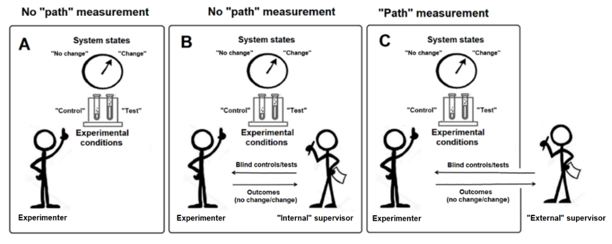
First, we will explain why Benveniste was convinced – with sound arguments – that he had discovered “something”. For this purpose, we will describe three experimental settings: open-label experiments, internal blinding and external blinding (Figure 1).

Open-label experiments. Figure 2 reports results on two devices that were used in parallel in 1992–1996. There was no blinding between the two measurements; these duplicate experiments were done in order to confirm the outcomes. To analyze these results, we do not care of the nature of the samples tested (C or T, high dilutions, electronic transmission, etc.) We only consider the concordance of the outcomes obtained with the two devices. We observe a high correlation of these measurement (the most probable pairs of outcomes are Δ⁰/Δ⁰ and Δ⁺/Δ⁺). The important point is for the pairs Δ⁺/Δ⁺. Indeed, these correlated pairs are a strong argument in favor of Benveniste’s theses. They indicate that there is “something” that occurs in these experiments. Whether one agrees or not with Benveniste’s views on the interpretation of these experiments, the source of correlations needs to be explored. This is precisely the purpose of the present article.

Internal blinding. The data of Table 1 indicate that these correlations persist after an internal blinding. Internal blinding means a blinding of labels of the samples to be tested (controls and tests) by a colleague who interacts with the experimenter in the laboratory (Figure 1). These data show that the pairs C/Δ⁰ and T/Δ⁺ are the most probable, thus strongly suggesting a direct relationship between labels and system states. Again, we understand why Benveniste defended his research with determination and why he could not resign himself to forgetting his results in a drawer as many suggested he should do [3].

External blinding. To share his experimental results and to convince his peers, Benveniste organized “public demonstrations” carried out in the presence of an audience of colleagues and observers who did not belong to the laboratory. These demonstrations were designed in order to give a “definitive” confirmation on the reality of these experiments and to establish their scientific interest. For this purpose, an experimental protocol was written and then a study report with all raw data was shared with participants [3]. During a typical session of demonstration, controls and tests were prepared (either high dilutions for the early demonstrations or computer files later) in another laboratory than Benveniste’s laboratory. These samples were prepared under supervision of all participants. Then, the labels of the control and test samples were replaced by a code by participants not belonging to Benveniste’s laboratory. Some samples were also kept unblinded to check that everything was fine in non-blinded conditions. Then, Benveniste’s team recovered all samples and tested them in its laboratory within the next days. After all measurements had been done, the outcomes (Δ⁰ and Δ⁺) corresponding to all blind samples were sent to the external supervisor who detained the code (Figure 1). This supervisor compared the two lists: list of labels (C vs. T) under a code name and list of outcomes (Δ⁰ vs. Δ⁺) and assessed whether outcomes were as expected (C associated to Δ⁰ and T associated to Δ⁺).

There was an internal blinding between the series of measurements for all these experiments (except November 4, 1996) in order to verify the consistency of the outcomes. Note that experiments done in 1996 were performed on two apparatus to confirm results as described in Figure 2.

A series of experiments with external blinding is presented in Table 2. It is easy to see that the relationship between labels and system states was lost in the experiments with external blinding. Indeed, in this table, square labels are not superimposed on round labels of the same color, but distributed at random. There was still an “effect”, i.e., the observation of changes of system state (Δ⁺), but not at the place where they were supposed to be.

To explain these oddities, Benveniste put forward various hypotheses (human errors for label allocation, water contamination, electromagnetic pollution, “remnant activity” in the apparatus, spontaneous “jumps of activity” from one sample to another, etc.) These mismatches prompted a technological race in which Benveniste engaged to rule out these supposedly disturbing external events. In contrast, in the present analysis, we consider that “successes” with open-label/internal blinding experiments (A and B in Figure 1) and “failures” with external blinding experiments (C in Figure 1) are the two faces of the same phenomenon. Actually, we think that these disturbing events are the scientific fact of this story. One important point must again be stressed. If Benveniste’s experiments were of no scientific interest, no change of the system state should be observed, whatever the experimental conditions.

In order to take into account all these aspects of Benveniste’s experiments – i.e., both “successes” and “failures” – we propose to abandon the idea of any role of water (“water memory” and its avatars) and to begin by revisiting the notion of relationship in experimental biology.

4. Theoretical Considerations on Relationship in Experimental Biology

To progress in the understanding of the phenomena reported by Benveniste’s team, we consider that all various procedures for diluting solutions or electronic stuff aimed to “transfer biological activity” make no sense. We state that they have no more value than a ritual or meaningless gesticulations.

We assume that the control and test conditions are physically identical and that their difference lies only in the respective labels (“control” or “test”) that they randomly or subjectively receive. Consequently, we consider that labels (“control” vs. “test”) and corresponding states of the biological system (“no change” vs. “change”) are independent variables. Two events are independent if the occurrence of one does not affect the probability of occurrence of the other. Yet a relationship between labels and system states was observed in Benveniste’s experiments. This is precisely the problem we have to solve.

For this purpose, we suppose a simple situation where labels (control, C; test, T) and system states (no change, Δ⁰; change of system state, Δ⁺) are independent variables with corresponding probabilities to be observed (Figure 3).

In this case, the law of total probability is:

P (C) × P (Δ⁰) + P (C) × P (Δ⁺) + P (T) × P (Δ⁰) + P (T) × P (Δ⁺) = 1

(Eq. 1)

with P (C) + P (T) = 1 and P (Δ⁰) + P (Δ⁺) = 1

For reasons that will appear later, we write:

i. P (C) = a² and P (T) = b² where a and b are real numbers

ii. P (Δ⁰) = cos²θ and P (Δ⁺) = sin²θ

With these conventions, the law of total probability described in Eq. 1 becomes:

(a.cosθ)² + (b.sinθ)² + (b.cosθ)² + (a.sinθ)² = 1

(Eq. 2)

We add δ = 2ab.cosθsinθ – 2ab.cosθsinθ = 0 to Eq. 2:

[(a.cosθ)² + (b.sinθ)² + 2ab.cosθsinθ] + [(b.cosθ)² + (a.sinθ)² – 2ab.cosθsinθ] = 1

(Eq. 3)

δ is equal to zero, but its addition allows to reorganize the equation with two remarkable identities:

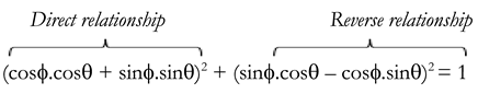
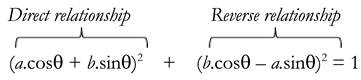
(a.cosθ + b.sinθ)2 + (b.cosθ – a.sinθ)2 = (a.cosθ)2 + (b.sinθ)2 + (b.cosθ)2 + (a.sinθ)2 = 1

(Eq. 4)

Eq. 4 shows that there are two possible writings of the law of total probability for two independent dichotomous random variables. We can also represent this equation graphically (Figure 4). We recognize a logical structure similar to an experiment where a photon “interferes with itself” such as in a two-slit Young’s experiment or in a Mach-Zehnder interferometer.

In the same logic as an interference experiment, the left side of Eq. 4 corresponds to the absence of path measurement (superposition with interference pattern), while the right side corresponds to path measurement (no interference pattern and labels associated randomly to system states). The real number a (resp. b) can be assimilated to a “probability amplitude” while a² (resp. b²) is the corresponding probability.

Therefore, there are two possible definitions of P (direct) according to path measurement or not:

P (direct)_I = (a.cosθ + b.sinθ)² if no path measurement

(Eq. 5)

P (direct)_II = (a.cosθ)² + (b.sinθ)² if path measurement

(Eq. 6)

Similarly, there are two possible definitions of P (reverse):

P (reverse)_I = (b.cosθ – a.sinθ)² if no path measurement

(Eq. 7)

P (reverse)_II = (b.cosθ)² + (a.sinθ)² if path measurement

(Eq. 8)

P (direct)_II can be also written by using conditional probabilities where P (X|Y) means probability of the event X knowing that the event Y has occurred:

P (direct)_II = a²cos²θ + b²sin²θ = P (C) × P (Δ⁰|C) + P (T) × P (Δ⁺|T)

(Eq. 9)

We see clearly with Eq. 9 how P (direct)_II is related to the “measurement of the path” (from a point of view outside the laboratory). It could be tempting to use conditional probabilities to rewrite Eq. 3. However, the difference δ of the “interference terms” is not egal to zero in all cases if conditional probabilities are considered:

δ = 2 a b \sqrt{P (Δ^{0} | C}) \sqrt{P (Δ^{+} | T}) - 2 a b \sqrt{P (Δ^{0} | T}) \sqrt{P (Δ^{+} | C})

(Eq. 10)

Indeed, δ = 0 only if P (Δ⁰|C) = P (Δ⁰|T) = P (Δ⁰) and if P (Δ⁺|T) = P (Δ⁺|C) = P (Δ⁺). In other terms, the two “interference terms” cancel each other only if labels (C or T) and system states (Δ⁰ or Δ⁺) are independent variables as initially postulated in Eq. 1. The “same randomness” must operate for system states, regardless of the paths C and T (see Figure 4).

Another important remark is for a particular case of Eq. 5 and Eq. 7:

If a = cosθ and b = sinθ, then P (direct)_I = 1 and P (reverse)_I = 0

(Eq. 11)

P (direct)_I = 1 means that each label C is associated with Δ⁰ and each label T is associated with Δ⁺. Note that there is no constraint on the order of the pairs (C, Δ⁰) and (T, Δ⁺); there is only a constraint on probabilities.

We can also represent Eq. 4 geometrically in a Cartesian coordinate system (Figure 5). In this representation, two bases, one for the labels (C and T) and the other for the relationships (direct and reverse), are necessary. Cosθ and sinθ are the “probability amplitudes” of Δ⁰ and Δ⁺, respectively. The two bases are related by a rotation matrix (with θ >0 in the clockwise direction):

(\begin{matrix} \cos θ & \sin θ \\ - \sin θ & \cos θ \end{matrix}) \times (\begin{matrix} a \\ b \end{matrix}) = (\begin{matrix} a \cos θ + b \sin θ \\ b \cos θ - a \sin θ \end{matrix})

(Eq. 12)

Each point can be projected (i.e., expressed) in one basis or the other (C/T or direct/reverse). The projection of a point of the unit circle leads to different results if projected directly to the direct/reverse basis or if projected first on the C/T basis and then on the direct/reverse basis. This last case (projection first on the C/T basis) is equivalent to a “which-path” measurement. For θ ≠ 0, direct/reverse relationships and control/test labels are said “non-commutative” variables because the final outcomes depend on the order of the projections.

5. Probabilities of Events vs. Probabilities of Their Relationships

The right part of Eq. 4 (a²cos²θ + b²sin²θ + b²cos²θ + a²sin²θ = 1) is the mathematical expression of the probabilities of events (selection of experimental conditions and measurements of system states) who are randomly associated. In contrast, the left part of Eq. 4 corresponds to the description of the possible relationships between these events:

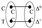
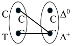
By varying the angle θ, all possible patterns of relationships can be described. For four values of θ, each label is associated to only one system state (Table 3 and Figure 6). For values of θ intermediate between two of these values of θ, mixtures of patterns are obtained.

Rotating the direct/reverse basis relatively to the C/T basis selects a pattern. Of course, the pattern number 2 is the one we are most interested in because it describes a direct relationship. Note however that there is no causality in this relationship. Indeed, each pair (one label associated with one system state) results from a selection among the possible random pairs. This filtering is the consequence of the interference terms.

6. Are All Random Systems Suitable?

Until now, we did not impose any condition for the experimental system. However, one may ask whether it would be possible to replace the biological system with any other system that produces randomness such as a random draw of black and white balls from a bag or a dice roll.

All experimental systems used in Benveniste’s experiments were biological systems involving cells, isolated organs or enzymatic reactions. Such systems are submitted – even at rest – to tiny random fluctuations. Therefore, in Figure 5, we can assume that the angle θ slightly fluctuates around zero. As a consequence, the probability to observe Δ⁺, which is P (Δ⁺) = (sinθ)², is not equal to zero, even though this probability is low. The transition of the system state from no change to change (Δ⁰ → Δ⁺) is therefore a possible event.

In contrast, suppose a bag full of many white balls (Δ⁰) and only a few black balls (Δ⁺). The probability to draw a black ball is low and white balls cannot transform into black balls. In other words, the transition of the system state from no change to change (Δ⁰ → Δ⁺) is not a possible event. Therefore, such a random system would not allow results comparable to those observed in Benveniste’s experiments.

7. What Physical Structures Support This Logic?

In the same way that a dice, a coin or a two-slit device is the physical support that governs the probabilities of the outcomes, we need now to define the physical structures that support the logic we propose.

Obviously, the physical support for Δ⁰ and Δ⁺ is the experimental biological system. Concerning control and test conditions (for example, samples of “informed water”), we have seen that we consider that they are physically identical and that the experimental differences are founded only on their denominations (“labels”). The latter have the meaning that the experimenter attributes to them and consequently the difference between control (C) and test (T) conditions is based on differences in the cognitive structures of the experimenter. Therefore, labels are subjective concepts which are embodied in the experimenter’s cognitive structures. To highlight this point, we can replace C with E^C and T with E^T which are the cognitive states of the experimenter (E) considering an experimental condition, either as a control condition or as a test condition, respectively. The law of total probability (Eq. 1) can be written as:

P (E^C) × P (Δ⁰) + P (E^C) × P (Δ⁺) + P (E^T) × P (Δ⁰) + P (E^T) × P (Δ⁺) = 1

with P (E^C) = a² and P (E^T) = b².

These remarks do not change Eq. 4. Simply we note that in the left part of Eq. 4:

The states of the experimenter’s cognitive structures and of the experimental system form an intertwined whole through their probability amplitudes so that P (direct) = (a.cosθ + b.sinθ)² and P (reverse) = (b.cosθ – a.sinθ)².

8. Emergence of Correlations between the Experimenter’s Cognitive Structures and the Experimental System

In Section 6, we have seen that Δ⁺, whose probability is the square of sinθ, is a possible event, but with a low probability. If we want to describe correlations between the experimental conditions (embodied in the experimenter’s cognitive structures and the states of the experimental system using Eq. 4, we need to explain how this equation can be in a non-trivial form (i.e., with a value of θ that deviates significantly from zero).

We propose that non-trivial values of θ have their origin in prior observations of repeated experiments where experimental conditions (labels) and system states exhibit a direct relationship. This process which can be considered as conditioning or learning, can be done by the experimenter observing, for example, a “classical” experiment. By “classical”, we mean an experiment with a “classical cause” (e.g., molecules of a biologically-active compound added to the biological system at the usual micromolar concentration). Note that in Benveniste’s laboratory the experimental systems were routinely used by the experimenters for “classical” experiments and biologically-active compounds were also used to verify that the systems were functioning correctly under “classical” conditions.

We note C=□, Δ⁰=○, T=■ and Δ⁺=● and define n₁, n_2, n₃ and n₄ (with n₁ + n₂ + n₃ + n₄ = N) as the numbers of trials where the experimenter records (□○), (■●), (□●) and (■○), respectively. Suppose now an experiment for which labels and system states are involved in a direct relationship, i.e., the series of outcomes that the experimenter records are, for example: (□○), (■●), (■●), (□○), (□○), (■●), (■●), (□○), (■●), etc. where the probability of C=□ is a² and the probability of T=■ is b².

When the number N of trials increases: n₁/N→ a², n₂/N → b², n₃/N→ 0 and n₄/N → 0

Since a² + b² = 1, the point Ω with coordinates

a = \sqrt{n_{1} / N}

and

b = \sqrt{n_{2} / N}

can be represented on the unit circle of Figure 7. Ω allows setting the position of the axis for “direct relationship” and the perpendicular axis for “reverse relationship”. It defines also the value of θ since sinθ = b. The abscissa of Ω on the direct axis is equal to a.cosθ + b.sinθ = a.a + b.b = 1 and therefore the ordinate on the reverse axis is b.cosθ – a.sinθ = b.a – a.b = 0. The two bases are related by a rotation matrix characterized by θ. Since, P (direct) = 1, correlations are therefore established between the experimental conditions (labels) and the experimenter’s cognitive structures.

Note that the underlying nature of the observed correlations does not matter (local cause or any other type of relationship).

In summary, the record of a statistical regularity shapes the intertwined whole constituted by the probability amplitudes of the states of the experimenter’s cognitive structures and of the experimental system. This statistical regularity is mathematically described by the direct/reverse basis with a non-zero value of θ.

8. Self-Sustained Correlations

The correlations established between the experimenter’s cognitive structures and the experimental system have an interesting property: they are self-sustained.

First, we write Eq. 4 by replacing a with cosφ and b with sinφ:

If θ=φ, it means that the intertwined whole composed of the probability amplitudes of the states of the experimenter’s cognitive structures and the experimental system is configured in such a way that the direct relationship is observed since P (direct) = 1. The consequence of this process is that the structuring of the intertwined whole influences the states of its parts. This is an example of downward causation defined as a causal relationship from higher level of a system to its lower-level parts. As a consequence, labels and system states obey the equation and organize themselves (regardless the order of labels) to form a direct relationship due to downward causation (Figure 8). Since a direct relationship is recorded, the value of θ is equal to φ, thus leading to P (direct) = 1. Then, labels and system states obey the equation, and so on. Recording of statistical regularity and downward causation concur to reinforce the non-zero value of θ.

9. Open-Label vs. Blind Experiments Explained

We will now examine how the formalism we describe could explain all aspects of Benveniste’s experiments.

Open-label experiments/internal blinding. Both the labels (C or T) and the system states (Δ⁰ or Δ⁺) are random events that are governed by their respective probabilities. The records of these events by the experimenter are measurements: during open-label experiments, the experimenter measures first the label (C or T) and then the system state (Δ⁰ or Δ⁺); during internal blinding, the experimenter measures first the system state and then the label (Figure 1). Internal blinding of labels can be performed by an automatic device or by a colleague present in the neighborhood of the experimenter. In this case, the blinding device (machine or human) is nothing more than a part of the experimental system.

We see in Eq. 4 that the order of probability amplitudes referring to labels and states of the system does not matter. Therefore, in our modelling, there is no difference in nature between open-label experiments and experiments with internal blinding.

In addition, we have seen that P (direct)_I = 1 and P (reverse)_I = 0 for sinθ = b and cosθ = a, thus showing that the probability amplitudes of labels and outcomes are merging when the correlation is maximal. C and Δ⁰ are combined in a single path (Path 1) and T and Δ⁺ are combined in another single path (Path 2) (Figure 9).

The internal blind experiments made always a deep impression on Benveniste’s team because they strongly suggested that the effects of high dilutions or digital biology were a tangible reality (“it works”). It was these experiments that convinced Benveniste that he had to persevere and that one day his theories and discoveries would be recognized. However, we have seen in this article that a logic other than a classical causal relationship is possible. This does not mean that causality is absent of this description, but causality operates at a higher level, i.e. at the level of the relationship. Internal blinding in Benveniste’s experiments should be no more surprising than internal blinding for a classical causal relationship. We must simply admit that what is at stake is not the physical composition of the sample to be tested – they are all identical – but its designation (label C or T). This label can be “measured” like any other parameter and a probability can be attributed to it.

External blinding. The external blinding – which constituted the “stunning block” described above – is simply explained by a “which-path” measurement with the laboratory in its ensemble being considered as an “interferometer”. Everything happens as if the external supervisor is making a measurement of the path from the outside by exchanging data on labels and system states (Figure 1). It is the external supervisor who provides the experimenter with coded samples to be tested.1 Finally, the external supervisor receives the records of the corresponding system states and, after unblinding, establishes whether the experiment is “successful”. Therefore, we can understand why these experiments were so disturbing for Benveniste's team. Indeed, even if these experiments were considered as “failures”, they nevertheless indicated that “something” happened because changes of the system were recorded (but randomly associated with C and T). The experiments seemed to be going “crazy”. In the “classical” and local approach of Benveniste’s team, there was no place for such outcomes. Therefore, external causes of disturbances were searched leading to a technological race for the “perfect” and indisputable experiment.

The experimental outcomes and underlying mathematics for open-label and blind experiments are summarized in Table 3.

10. Discussion

In this analysis of Benveniste’s experiments, details on the biological models and the different methods used to “inform” water are left aside. Only the logical structure of the outcomes is analyzed. In order to review these experiments with a renewed perspective, a radical choice has been done by considering that control and test conditions that were evaluated in Benveniste’s experiments differed only by their specific names (labels). Indeed, we previously noted that whatever the process used to inform water (high dilutions, direct electromagnetic transmission, record on a computer memory, etc.), the effect size whatever the experimental system was of the same order of magnitude [3,22]. This suggested that an alternative unique explanation – independent of the different methods and devices used – might be at work. This radical choice seems to make any explanation of Benveniste's experiments even more problematic. Indeed, how could a relationship be observed if the samples tested are all physically comparable to simple controls?

For this purpose, the mathematical formalism starts from scratch with the definition of the total probability law for two dichotomous independent variables, namely labels (which designate the experimental conditions, either control or test) and the corresponding system states. We easily obtain Eq. 4 where the left and right parts can be considered as complementary. The two parts cannot be considered simultaneously, but both are necessary to understand the logic of Benveniste’s experiments. The formalism requires a description from the outside where the laboratory and its content behave with the same logic as an “interferometer”. The “causality” of the relationship described by the present formalism is only apparent since measurement of the “path” destroys the correlations: labels (C vs. T) are then randomly associated with system states (no change vs. change). This is precisely the description of the Benveniste’s stumbling block.

The model we propose uses probability amplitudes (with an imaginary art equal to zero) which is more common in a quantum physics context. We also make a parallel with the two-slit Young’s experiment. Nevertheless, there is no quantum physics in this model. In the same way quantum-like logic has been used with success in the field of experimental psychology in a new approach named quantum cognition. Cognitive processes such as decision making, judgment, memory, reasoning, language or perception, not adequately described by “classical” probabilities, are modelled with mathematical quantum-like tools, in particular probability amplitudes, thus better fitting experimental data [23,24]. In quantum cognition, combining abstract concepts is associated to quantum-like phenomena such as superposition and interferences. However, in quantum cognition, all processes are supposed to be limited to brain, while our modelling involves not only the experimenter’s cognitive structures, but also an experimental biological system. Nevertheless, there is nothing magical since there is no “action” of the mental structures on the experimental system. Indeed, if one tries to demonstrate a causal relationship or to use the correlations in a causal way to perform an action (e.g., giving an order or sending a message), the direct relationship between the experimenter and the system breaks down.

The source of the correlations between the experimenter and the experimental system is to be found in the complementarity of labels and system states as separate “objects” on the one hand and their relationship on the other hand. A parallel can be drawn with the wave-particle duality where either waves or particles are detected depending on the measuring device. Particles and waves are classical concepts that we can apprehend with our measurement tools, our senses, our language and our usual concepts to describe reality. Depending on the experimental context, either wave or particle descriptions are appropriate (they are said complementary). Thus, light behaves as waves when it does not interact with matter and behaves as particles (i.e., photons) when it interacts with matter (for example, with a measurement apparatus). These two descriptions – particles or waves – are incompatible pictures of reality (we cannot think about them simultaneously). Nevertheless, both descriptions are necessary to account for quantum or quantum-like phenomena when we use our usual concepts about reality. In the formalism of this article, the experimental events (C, T, Δ⁰ and Δ⁺) are described as “particles” while the relationship between them is described as “wave”. Thus, P (direct)_II = (a.cosθ)² + (b.sinθ)² is a “particle” description of the experimental situation; P (direct)_I = (a.cosθ + b.sinθ)² is a “wave” description which differs from P (direct)_II by the interference term 2ab.cosθsinθ. Interferences are characteristic of wave interactions that can be constructive or destructive according to the values of the amplitudes of the waves that are superposed at a given point. Thus, to calculate P (direct)_I, the two amplitudes a.cosθ and b.sinθ are added (amplitudes can be positive or negative). In quantum or quantum-like formalism, probability amplitudes have no intuitive correspondence in the real world. Indeed, these “waves” are not “waves of matter”, but “waves of probability”. The connection with reality is done via probabilities, which are obtained after squaring the sum of all probability amplitudes that concur to the outcome (direct or reverse relationship in the present case).

The crucial element of our description of Benveniste’s experiments is how to explain the emergence of the direct/reverse basis. For this purpose, we propose that the recording of a statistical regularity (“classical” relationship, for example) shapes the the intertwined whole constituted by the probability amplitudes of the states of the cognitive structures of the experimenter “extended” with the experimental system. This process can be described as learning or conditioning. It is important to underscore that this combination of a label with the corresponding system state is not a simple addition or juxtaposition. Indeed, during this process, everything happens as if the relationship were recognized as such (i.e., independently of its constitutive elements). These considerations are reminiscent of Gestalt theory. According to this theory, objects are perceived as a whole or as a form (Gestalt) by the mind and not as the sum of their parts; the whole has therefore its own independent existence [25,26].

The automation of the experimental process is not necessarily the solution to avoid an “experimenter effect”. As previously said, Benveniste’s team set up a robot analyzer (based on fibrinogen coagulation) that required only to push one switch to launch an experiment. The choice of control and test conditions was randomized by a computer and the experimenter was informed of the results when the experiment was finished. An expertise of this apparatus was mandated by the DARPA and was performed in Summer 2001 in a US laboratory at Bethesda [21]. In their report, the multidisciplinary team concluded that they did not observe anything abnormal about the robot analyzer and that the experiments they supervised in the presence of Benveniste's team seemed to confirm the concepts of “digital biology”. They noted, however, that the presence of the experimenter dedicated to these experiments seemed to be necessary for the expected results to be observed. They also reported that after the departure of Benveniste’s team, no effect at all (i.e., no change of system state whatever the label) could be observed using this robot. The existence of unknown “experimenter factors” was suggested by some members of the supervisory team [21]. The final conclusion was that the alleged phenomenon based on “digital biology” was not replicable. Note that this failure was different from the failures reported above with external blinding. Here, what has been raised as a concern in the DARPA expertise was the requirement of a trained/conditioned experimenter to record a change of the system state. The relationship between conditioned vs. non-conditioned experimenter, on the one hand, and “success” vs. “failure” of the experiment, on the other, appears to be the actual causal relationship that was at work during Benveniste’s experiments.

With this latest episode of DARPA expertise, which concludes the “water memory” saga, it is unreasonable to persist in considering – as Benveniste and his supporters did – that high dilutions, “water memory” or “digital biology” constituted a major breakthrough in biology and medicine. If plain causal relationships were really at work, the existence of “water memory” and its avatars would certainly have been demonstrated without the difficulties we described. It is even possible that such non-classical correlations between labels and biological systems occur in other laboratories unwittingly to the experimenters who think that they have evidenced a “real” (causal) relationship. We can also hypothesize that the lack of replicability of certain experiments could be explained by such a non-classical phenomenon. If this type of phenomenon is suspected, experiments with an external supervisor can help clarify. This modelling could also be useful in the description of the placebo effect or in some alternative medicines.

In conclusion, we have seen in this article how simple considerations based on probability theory led to describe non-classical correlations involving the experimenter. This probabilistic modelling allows to propose an alternative explanation to Benveniste’s experiments where water plays no role and where the place of the experimenter is central. All aspects of Benveniste’s experiments are taken into account in this modelling, including the weird stumbling block. This obstacle prevented proving the causal relationship between the information supposedly stored in water and the corresponding “effect” observed on the biological system. Nevertheless, because Benveniste persisted in his quest for the definitive experiment that would convince everyone, he has transmitted to us a corpus of well-conducted experiments. For this reason, we must express our gratitude to him. He was pursuing what seems today a chimera, but his experimental data allow us to suggest the possible emergence of non-classical correlations between an experimenter and a biological system. Although these correlations mimic classical relationships, they are not causal Causality is not absent, however, but the cause of these correlations is at the level of the entire system, not at the level of its elements.

Funding

The author received no financial support.

Declaration of conflicting interests

The author declares that there is no conflict of interest.

References

“Serendipity.” Merriam-Webster.com Dictionary, Merriam-Webster, https://www.merriam-webster.com/dictionary/serendipity.
Beauvais F. L’Âme des Molécules – Une histoire de la "mémoire de l’eau" (2007) Collection Mille Mondes. https://www.researchgate.net/publication/280625214_L'Ame_des_Molecules_-_Une_Histoire_de_la_Memoire_de_l'Eau.
Beauvais F. Ghosts of Molecules – The case of the “memory of water” (2016) Collection Mille Mondes. https://www.researchgate.net/publication/280625430_Ghosts_of_Molecules_-_The_Case_of_the_Memory_of_Water.
Benveniste J. Ma vérité sur la mémoire de l'eau. Paris: Albin Michel; 2005.
de Pracontal M. Les mystères de la mémoire de l'eau. Paris: La Découverte; 1990.
Thomas Y. The history of the Memory of Water. Homeopathy. 2007;96:151-7. [CrossRef]
Poitevin B. The continuing mystery of the Memory of Water. Homeopathy. 2008;97:39-41. [CrossRef]
Schiff M. The Memory of Water: Homoeopathy and the Battle of Ideas in the New Science. London: Thorsons Publishers; 1998.
Alfonsi M. Au nom de la science. Paris: Bernard Barrault; 1992.
Ragouet P. The Scientific Controversies and the Differenciated Nature of Science. Lessons from the Benveniste Affair. L’Année sociologique. 2014;64:47-78.
Ball P. H2O: A biography of water: Weidenfeld & Nicolson; 1999.
Kaufmann A. The affair of the memory of water. Towards a sociology of scientific communication. Réseaux The French journal of communication. 1994;2:183-204. [CrossRef]
Maddox J, Randi J, Stewart WW. "High-dilution" experiments a delusion. Nature. 1988;334:287-91. [CrossRef]
Benveniste J. Benveniste on Nature investigation. Science. 1988;241:1028. [CrossRef]
Benveniste J, Aïssa J, Litime MH, et al. Transfer of the molecular signal by electronic amplification. Faseb J. 1994;8:A398.
Aïssa J, Jurgens P, Litime MH, et al. Electronic transmission of the cholinergic signal. Faseb J. 1995;9:A683.
Benveniste J, Jurgens P, Aïssa J. Digital recording/transmission of the cholinergic signal. Faseb J. 1996;10:A1479.
Benveniste J, Jurgens P, Hsueh W, et al. Transatlantic transfer of digitized antigen signal by telephone link. J Allergy Clin Immunol. 1997;99:S175.
Benveniste J, Aïssa J, Guillonnet D. Digital biology: specificity of the digitized molecular signal. Faseb J. 1998;12:A412.
Benveniste J, Aïssa J, Guillonnet D. The molecular signal is not functional in the absence of "informed" water. Faseb J. 1999;13:A163.
Jonas WB, Ives JA, Rollwagen F, et al. Can specific biological signals be digitized? FASEB J. 2006;20:23-8.
Beauvais F. Emergence of a signal from background noise in the "memory of water" experiments: how to explain it? Explore (NY). 2012;8:185-96.
Busemeyer J, Bruza P. Quantum models of cognition and decision: Cambridge University Press; 2012.
Bruza PD, Wang Z, Busemeyer JR. Quantum cognition: a new theoretical approach to psychology. Trends Cogn Sci. 2015;19:383-93. [CrossRef]
Jakel F, Singh M, Wichmann FA, et al. An overview of quantitative approaches in Gestalt perception. Vision Res. 2016;126:3-8. [CrossRef]
Amann A. The Gestalt problem in quantum theory: generation of molecular shape by the environment. Synthese. 1993;97:125-56. [CrossRef]

1	By doing so, the experimenter prevents the random selection of each label (C or T) and conditional probabilities apply (See Eq. 9). This action is equivalent to closing one of the two slits in Young’s experiment.

Figure 1. Configurations for (A) open-label, (B) “internally” blinded and (C) “externally” blinded experiments. The “internal” or “external” supervisor provides the experimenter with “control” and “test” samples whose labels have been masked (blind controls/tests). After the experiment is done, the experimenter returns to the supervisor the outcomes which have been obtained (change or no change of system state noted Δ⁰ and Δ⁺, respectively) for each control or test. The supervisor assesses the rate of “success” of the experiment (i.e., how many direct relationships have been obtained with the masked samples: “control” associated with “no change” or “test” associated with “change”).

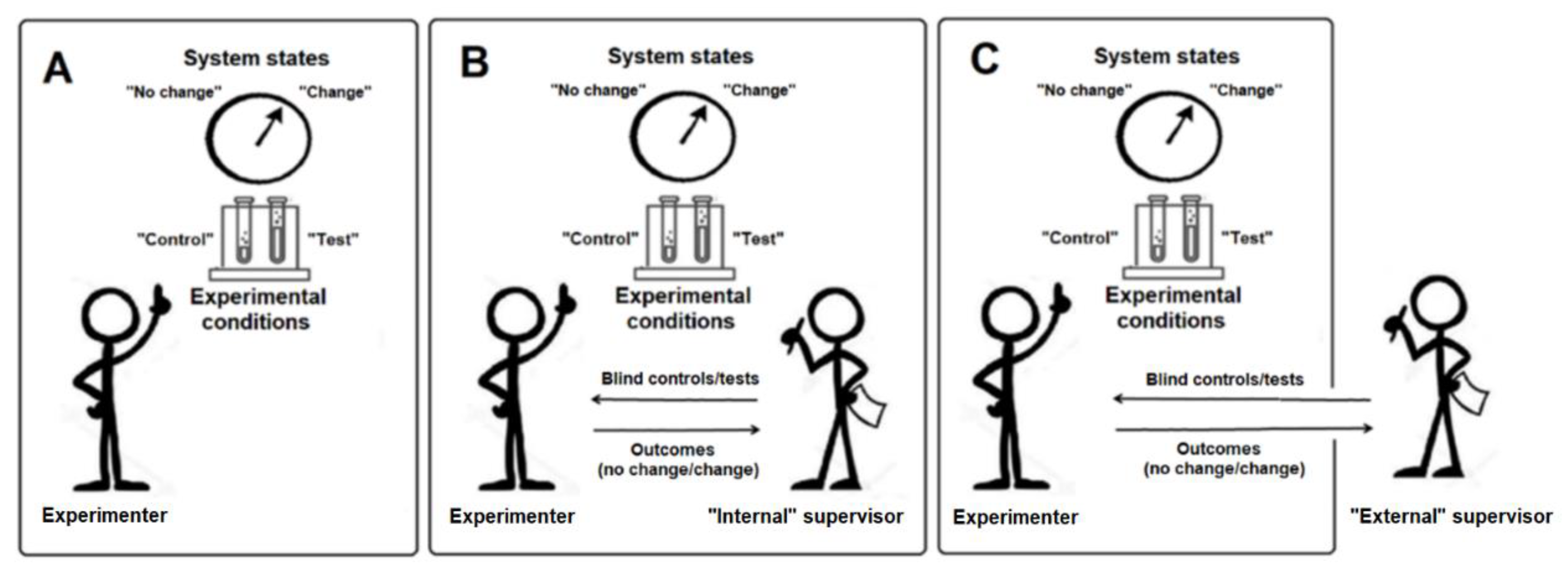
Figure 2. Open-label experiments made in duplicate on two experimental systems (dates: 1992–1996; experimental model: changes of coronary flow in isolated rodent heart; N=574 pairs of measurements) [22]. (a) In this figure we do not care about the label (control or test), only the concordance of the system states (Δ⁰ or Δ⁺) on the two devices matters. We also do not care of the method used by Benveniste’s team to produce controls and tests (high dilutions, electronic transmission, digital biology, etc.) The data obtained in devices A and B appear to be highly correlated. (b) If the value measured on the device A is < 10% (no change; Δ⁰), then the probability of a value < 10% on device B is 0.93. (c) If the value measured on the device A is ≥10% (change; Δ⁺), then the probability of a value ≥ 10% on device B is 0.89. Note that scales are logarithmic.

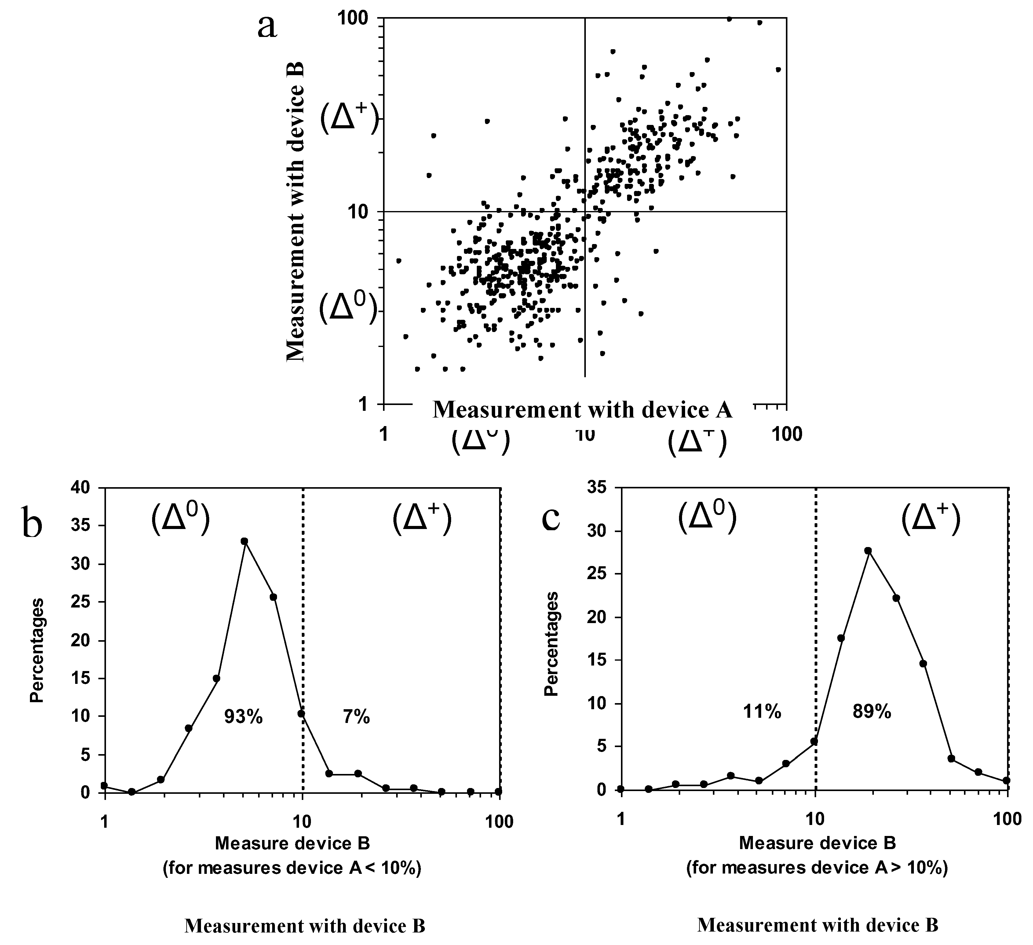
Figure 3. Law of total probability for two sets of independent variables: experimental conditions (control C vs. test T) and system states (no change of system state, Δ⁰ vs. change of system state, Δ⁺). According to the law of total probability, the sum of the probabilities of the four possible branches is equal to one. Note that P (C) + P (T) = 1 and P (Δ⁰) + P (Δ⁺) = 1.

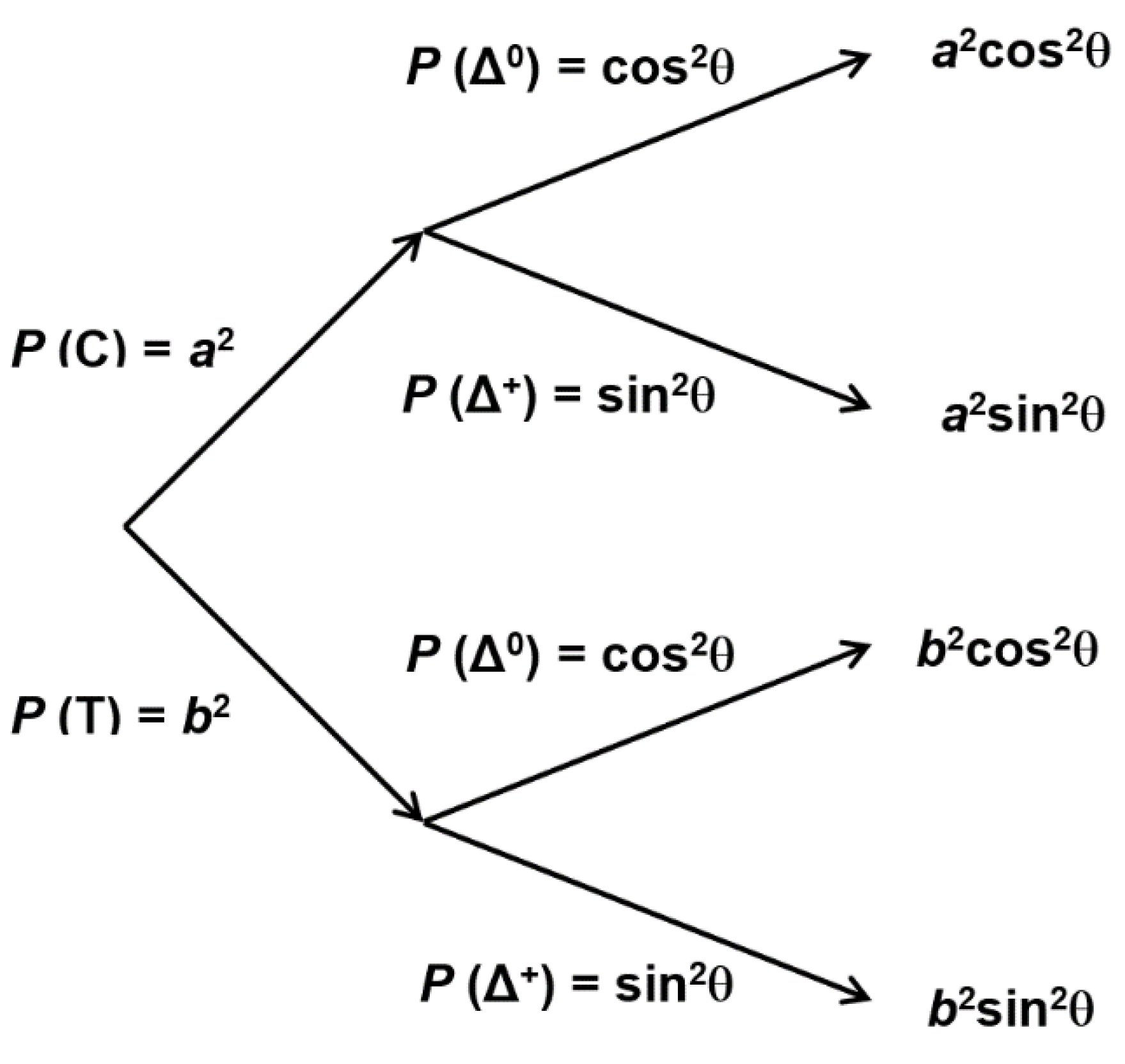
Figure 4. Graphical representation of Equation 4. Probabilities of direct and reverse relationships are calculated as the square of the sum of the probability amplitudes of the two possible paths: P (direct)_I = (a.cosθ + b.sinθ)² and P (reverse)_I = (b.cosθ – a.sinθ)². In contrast, when a path measurement is performed, probabilities are calculated as the sum of the squares of the probability amplitudes of paths: P (direct)_{II =} a²cos²θ + b²sin²θ and P (reverse)_{II =} b²cos²θ + a²sin²θ.

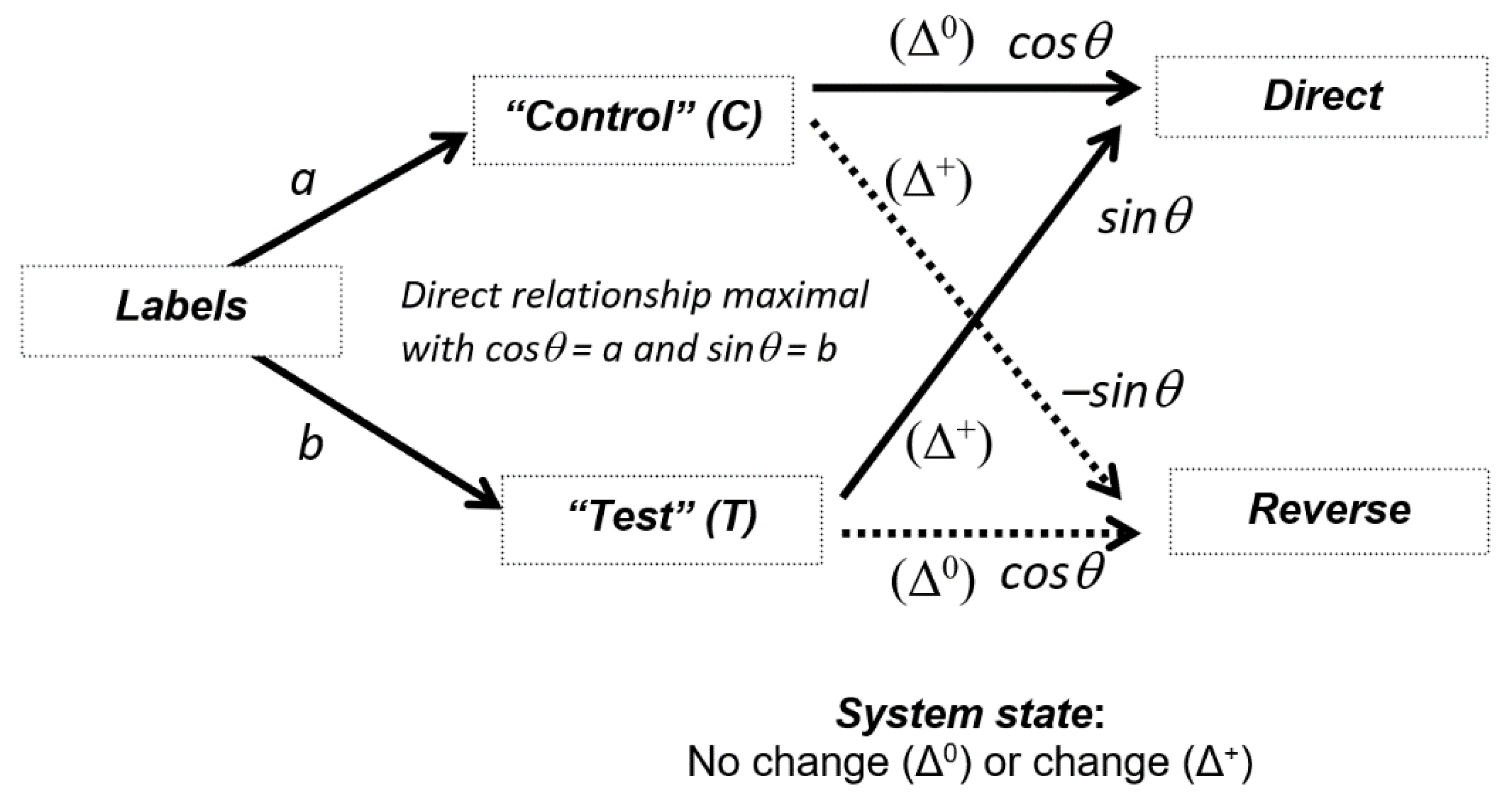
Figure 5. Representation of Equation 4 in a Cartesian coordinate system. The point Ω with coordinates a and b in C/T basis has coordinate a.cosθ + b.sinθ on the direct relationship axis; the associated probability is therefore (a.cosθ + b.sinθ)². If the relationship is assessed separately for C and T (path measurement), the coordinates on the direct relationship axis are a.cosθ for C and b.sinθ for T, with the corresponding probability for direct relationship equal to (a.cosθ)² + (b.sinθ)². For clarity, projections for reverse relationship are not presented on the figure.

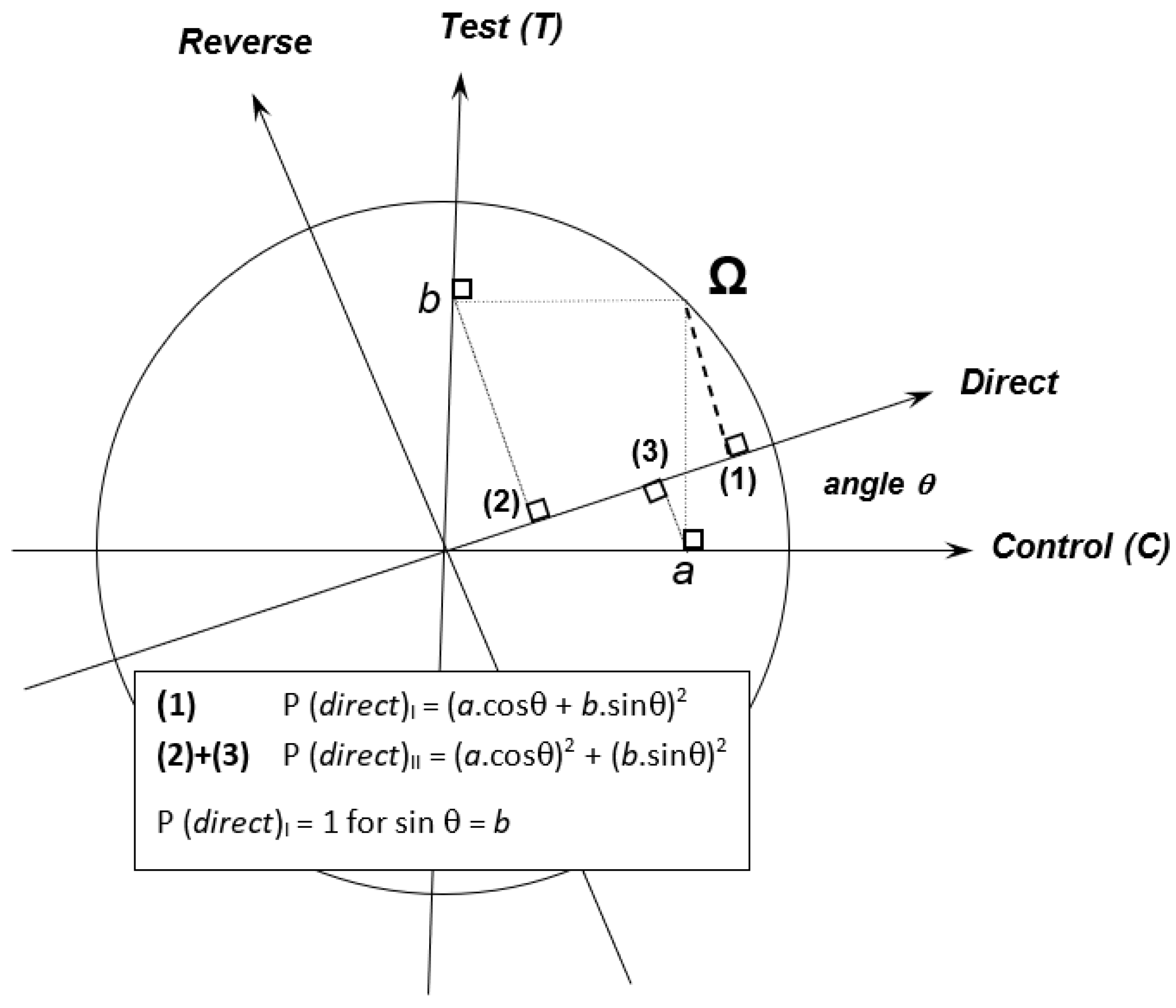
Figure 6. Patterns of relationships according to the angle θ. The direct/reverse basis is obtained after rotating the C/T basis by an angle θ. The four patterns from (1) to (4) corresponds to four values for the angle θ: Π/2, φ, 0 and φ + Π/2 (φ is defined as sinφ = b and cosφ = a). For this figure, the “direct” axis has been positioned on the point (2) such as θ = φ. For θ = φ, the direct relationship is maximal and mimics a causal relationship where C is associated to Δ⁰ and T is associated to Δ⁺.

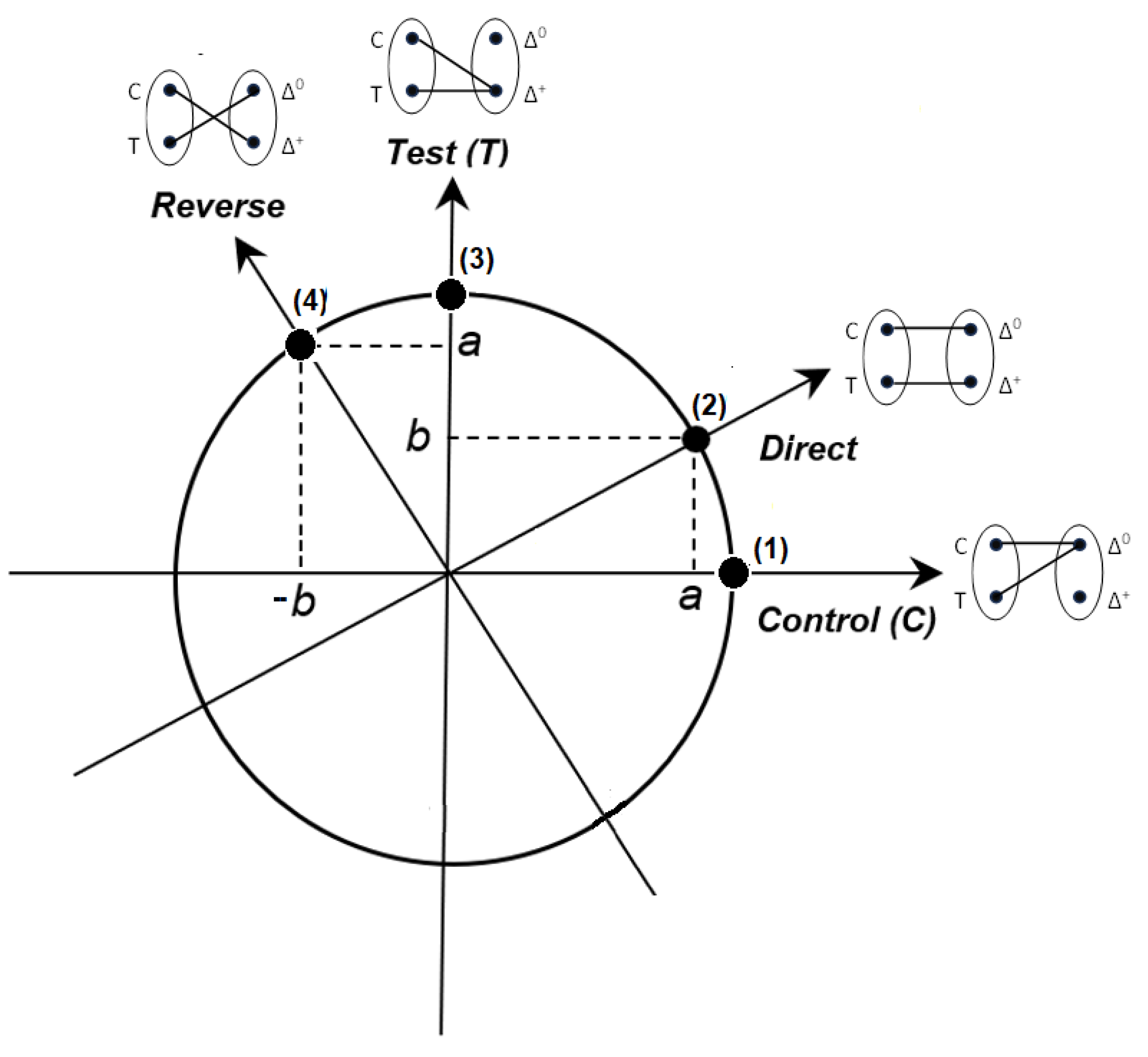
Figure 7. Setting of the direct/reverse basis. (A) After repeated experiments (e.g. with a “classical” biologically-active compound), the label C (probability a²) is systematically associated to Δ⁰ and T (probability b²) is systematically associated to Δ⁺ (statistical regularity). This statistical regularity can be represented on the unit circle by the point Ω with coordinates a and b which are real numbers. (B) Ω is not an experimental result, but is a limit (

\sqrt{n_{1} / N} \to a

;

\sqrt{n_{1} / N} \to b

) which integrates results of repeated correlation measurements observed between labels and system states. This point allows defining a new basis (direct/reverse). In this new basis, the direct relationship is recognized as such, independently of the elements (labels and system states) that permitted to define it.

\sqrt{n_{1} / N} \to a

;

\sqrt{n_{1} / N} \to b

Figure 8. Self-sustained correlations. Labels C (□) and T (■) – which are embodied in the experimenter’s cognitive structures – are characterized by the angle φ of their probability amplitudes (cosφ=a and sinφ=b) and states Δ⁰ (○) and Δ⁺ (●) of the experimental system are characterized by the angle θ of their probability amplitudes (cosθ and sinθ). If θ = φ, downward causation is the source of correlations between labels and system states. Then, recording of statistical regularity reinforces the mathematical equality between θ and φ, which in turn guarantees the association of labels and system states in a direct relationship (via downward causation).

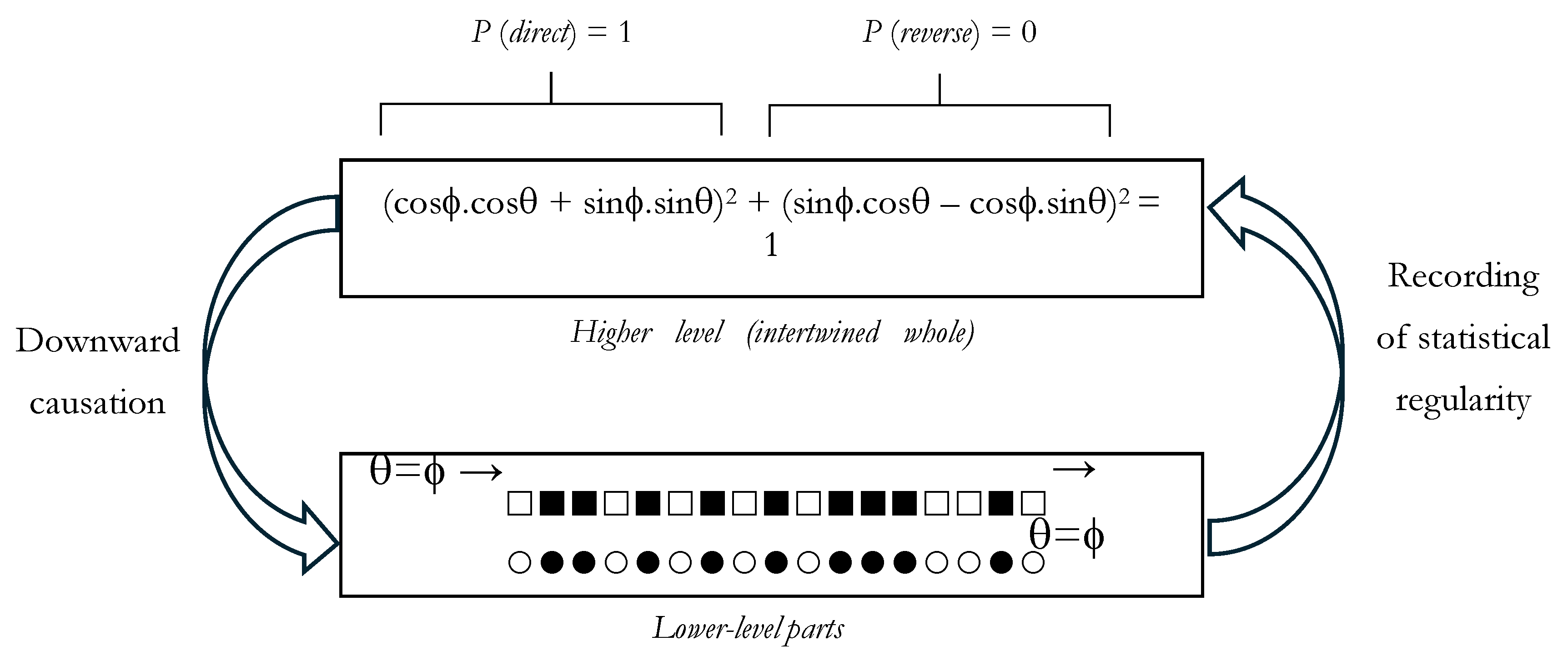
Figure 9. Consequences of self-sustained correlations in open-label, “internally” blinded and “externally” blinded experiments. (A) The probability of a direct relationship is maximal with a = cosθ and b = sinθ. Any couple (a, b) defines an angle φ and P (direct) _I = 1 if θ = φ. In this case, C and Δ⁰ are combined in a single path (Path 1) and T and Δ⁺ are combined in another single path (Path 2) with P (direct)_I = (a.a + b.b)² = 1 (no path measurement; open-label experiments or “internal” blinding) and P (direct)_II = (a.a)² + (b.b)² (path measurement; external blinding). (B) Geometrical representation of the two bases (Direct/Reverse and Path 1/Path 2) on a unit circle.

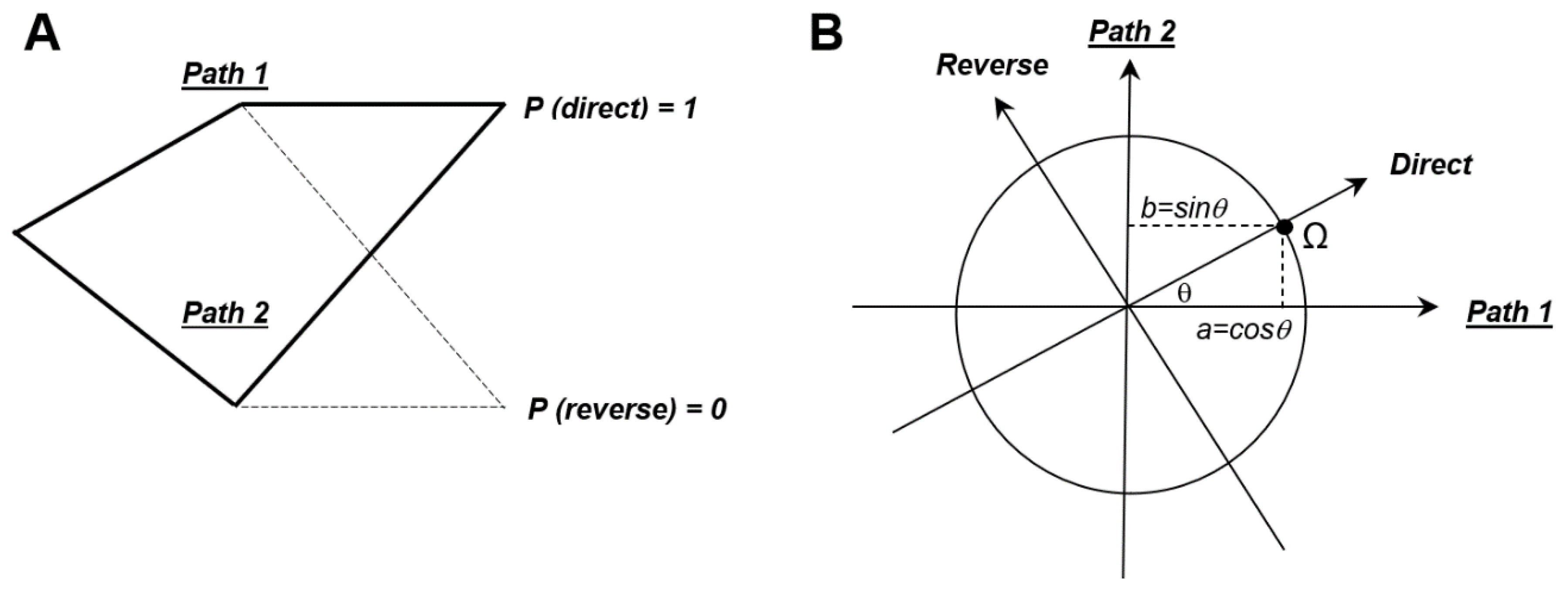
Table 1. Experiments with internal blinding (dates: 1993–1997; experimental model: changes of coronary flow in isolated rodent heart) [22].

Experimental situations	N	System states after internal blinding
Experimental situations	N	No change (Δ⁰)	Change (Δ⁺)
Interim blinding between 1st and 2nd measurement of the same sample
No change (Δ⁰) for 1st measurement	50	96% (2nd measurement)	4% (2nd measurement)
Change (Δ⁺) for 1st measurement	28	7% (2nd measurement)	93% (2nd measurement)
Blind labels
Label “Control”	68	88%	12%
Label “Test”	58	19%	81%

Table 2. “Digital biology” experiments with external blinding (dates: 1996-1997; experimental model: changes of coronary flow in isolated rodent heart) [3]. In these experiments (public demonstrations with external supervisor), system states are distributed at random in contrast with open-label or internal blinding experiments presented in Figure 2 and Table 1). Therefore, no relationship can be established between labels and system states. If a causal relationship existed, one would expect square labels to be superimposed on round labels of the same color. These “mismatches” were considered by Benveniste as experimental failures. In the present analysis, we consider that “successful” and “failed” experiments are the two faces of the same phenomenon. Note that the observation of changes of state (noted ●), whatever their place, requires an explanation. Indeed, according to current scientific knowledge, we would expect to observe only no change of system state (○-○-○-○-○-○-○, etc.) The scientific context and the experimental details of these experiments can be found in [3].

February 27, 1996	Labels (□ = C, ■ = T)	□-■-■-□-■-□-■-□-■-□-■-■-■-■-■-■-■-□
February 27, 1996	States (○ = Δ⁰, ● = Δ⁺)	●-○-●-●-●-○-●-●-○-●-●-○-●-●-○-●-●-○
May 7, 1996	Labels (□ = C, ■ = T)	■-□-■-□-□-■-□-■-□-■
May 7, 1996	States (○ = Δ⁰, ● = Δ⁺)	○-●-○-●-○-●-○-●-○-●
June 12, 1996* (two parts)	Labels (□ = C, ■ = T)	□-□-■-□-■-■-■-■ / ■-□-■-■-■-■-□-□
June 12, 1996* (two parts)	States (○ = Δ⁰, ● = Δ⁺)	○-●-○-○-●-○-○-● / ●-○-○-●-○-○-●-○
September 30, 1996*	Labels (□ = C, ■ = T)	■-□-□-□-□-■-■-□-□
September 30, 1996*	States (○ = Δ⁰, ● = Δ⁺)	○-●-●-○-●-●-○-○-●
November 4, 1996	Labels (□ = C, ■ = T)	■-■-□-■-■-□-■-□-□-□
November 4, 1996	States (○ = Δ⁰, ● = Δ⁺)	●-○-○-●-○-○-○-●-○-●
December 4, 1996*	Labels (□ = C, ■ = T)	□-■-■-□-□-■-□
December 4, 1996*	States (○ = Δ⁰, ● = Δ⁺)	●-○-○-○-●-○-●
September 27, 1997*	Labels (□ = C, ■ = T)	□-□-■-□-□-□-■-■-■-■
September 27, 1997*	States (○ = Δ⁰, ● = Δ⁺)	●-○-●-○-●-●-○-○-●-●

* The number of controls and tests to be evaluated was not known from the experimenter.

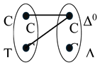
Table 3. Patterns of the four possible relationships (with only one system state associated to each label) according to the value of θ.

Patterns of relationships

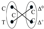(1) Only Δ⁰	(2) All direct	(3) Only Δ⁺	(4) All reverse
θ = 0	θ = φ ^a	θ = Π/2	θ = φ + Π/2
P (direct) = a²	P (direct) = 1	P (direct) = b²	P (direct) = 0
P (reverse) = b²	P (reverse) = 0	P (reverse) = a²	P (reverse) = 1

^a φ is defined as sinφ = b and cosφ = a.

Table 3. Summary of experimental results according to the conditioning of the experimenter and path measurement. Non-commutativity of the variables (labels and systems states) is the underlying logic explaining the outcomes of the different experimental situations.

	No conditioned experimenter	Conditioned experimenter
	No conditioned experimenter	No path measurement by external supervisor	Path measurement by external supervisor
Order of the experiments Labels ( □ = C,■ = T ) States (○ = Δ ⁰,● = Δ ⁺)	1 2 3 4 5 6 7 8 9 10 etc. □ ■ ■ □ ■ □ ■ □ ■ □ ○ ○ ○ ○ ○ ○ ○ ○ (●) ○	1 2 3 4 5 6 7 8 9 10 etc. □ ■ ■ □ ■ □ ■ □ ■ □ ○ ● ● ○ ● ○ ● ○ ● ○	1 2 3 4 5 6 7 8 9 10 etc. □ ■ ■ □ ■ □ ■ □ ■ □ ● ○ ● ● ● ○ ○ ● ○ ○
Comments	● is a possible but rare event	● is no more a rare event	● at random places (interpreted as “jumps of activity” by Benveniste’s team)
P (direct)	≈ P (□) = a²	= (a.cos θ + b.sin θ )² = 1 ^a (probability amplitudes add up)	= ( a .cos θ )² + (b.sin θ )² = a⁴ + b⁴
P(reverse)	≈ P (■) = b²	= (b.cosθ – a.sinθ)² = 0 ^a (probability amplitudes cancel)	= (b.cosθ)² + (a.sinθ)² = 2a²b²

^a For cosθ = a and sinθ = b.

Disclaimer/Publisher’s Note: The statements, opinions and data contained in all publications are solely those of the individual author(s) and contributor(s) and not of MDPI and/or the editor(s). MDPI and/or the editor(s) disclaim responsibility for any injury to people or property resulting from any ideas, methods, instructions or products referred to in the content.

© 2024 by the authors. Licensee MDPI, Basel, Switzerland. This article is an open access article distributed under the terms and conditions of the Creative Commons Attribution (CC BY) license (http://creativecommons.org/licenses/by/4.0/).

Copyright: This open access article is published under a Creative Commons CC BY 4.0 license, which permit the free download, distribution, and reuse, provided that the author and preprint are cited in any reuse.

Downloads

383

Views

253

Comments

Subscription

Notify me about updates to this article or when a peer-reviewed version is published.

MDPI Initiatives

Important Links

Choose an area of interest and we will send you notifications of new preprints at your preferred frequency.

Disclaimer

Benveniste’s Experiments and the So-Called “Water Memory” Phenomenon: an Example of Serendipity? Investigation and Experiments

Abstract

Keywords:

Subject:

1. Introduction

2. Causal Relationships in Experimental Biology

3. When the Scientific Interest Is Not Where It Was Supposed to Be

4. Theoretical Considerations on Relationship in Experimental Biology

5. Probabilities of Events vs. Probabilities of Their Relationships

6. Are All Random Systems Suitable?

7. What Physical Structures Support This Logic?

8. Emergence of Correlations between the Experimenter’s Cognitive Structures and the Experimental System

8. Self-Sustained Correlations

9. Open-Label vs. Blind Experiments Explained

10. Discussion

Funding

Declaration of conflicting interests

References

MDPI Initiatives

Important Links

Subscribe