
Submitted:
25 September 2026
Posted:
28 September 2026
You are already at the latest version
Abstract
Artificial intelligence (AI) is widely expected to raise productivity, yet whether its diffusion is already lifting growth in emerging economies is unclear. We assemble a panel of 42 emerging economies over 2010–2023 and construct an AI Adoption Capacity Index (AACI) that combines five indicators of connectivity, compute and data infrastructure, competency and technological context through principal component analysis. The index is validated against AI patenting (Spearman ρ = 0.59). Two-way fixed-effects growth regressions with Driscoll–Kraay standard errors find no positive short-run association between the AACI and GDP per capita growth: the preferred estimate is −1.07 percentage points per standard deviation (p = 0.12). System GMM estimates are negative and significant, but their over-identification diagnostics are marginal, and a peer-diffusion instrument is too weak to be informative. The average hides systematic heterogeneity. The AACI’s growth effect rises with tertiary enrolment (interaction p = 0.02), and it is more negative in economies with below-median initial income. Using Penn World Table data, total factor productivity and labour productivity growth respond negatively in the short run. Together, these patterns match a productivity J-curve, in which building AI capacity absorbs resources before complementary skills and intangibles pay off. They do not support the view that AI capacity is already a growth engine for emerging economies. The results caution against treating AI infrastructure as a substitute for human-capital deepening and point to absorptive capacity as the binding constraint on AI-led convergence.
Keywords:
artificial intelligence
; economic growth
; emerging economies
; technology diffusion
; absorptive capacity
; dynamic panel data
; productivity J-curve
1. Introduction
Artificial intelligence has become the leading candidate for the next general-purpose technology. Estimates of its macroeconomic payoff nevertheless differ by an order of magnitude. Task-based calculations for the United States put the ten-year gain in total factor productivity (TFP) at around 0.7% [1]. Alternative aggregation and diffusion assumptions yield considerably larger gains, of the order of several tenths of a percentage point of TFP growth per year [2,3]. For emerging and developing economies the uncertainty is larger still. Institutional assessments consistently conclude that advanced economies are both more exposed to AI and better prepared to exploit it [4,5,6]. This raises the prospect that AI could widen, rather than narrow, global income gaps [7,8].
Most existing evidence is either ex ante (simulation and exposure-based projections) or concentrated on advanced economies and firms [9,10]. Econometric evidence on whether AI capacity has actually been associated with faster growth in emerging economies remains scarce. A recent systematic review of 194 studies on AI and economic development finds the literature fragmented and context-dependent, with Africa and Latin America markedly under-represented [11]. Studies that do estimate cross-country panel relationships typically proxy AI with patents, a measure of AI invention, which is heavily concentrated in a handful of countries [12]. That measure says little about adoption in economies that mainly import rather than produce AI technology.
This paper asks a direct question: does AI adoption drive economic growth in emerging economies? We make four contributions.
- 1.
- Measurement. We construct an annual AI Adoption Capacity Index (AACI) for 42 emerging economies over 2010–2023, following the World Bank’s “4Cs” framework (connectivity, compute, competency, context) [8]. The index is built by principal component analysis (PCA) from five internationally comparable indicators, and we validate it against AI patenting [13].
- 2.
- Identification. We estimate growth regressions with two-way fixed effects and Driscoll–Kraay inference [14]. We address dynamic-panel bias and reverse causality with system GMM using collapsed instruments and Windmeijer-corrected standard errors [15,16,17], and complement it with a peer-diffusion instrumental-variable (IV) design.
- 3.
- Mechanisms. We test for complementarities with human capital, for heterogeneity by initial development, and for productivity channels using Penn World Table (PWT) TFP [18].
- 4.
- Transparency. Every estimate is produced by an openly documented pipeline from public data. We report null and fragile results alongside significant ones.
The answer is: not yet, and not unconditionally. We find no evidence that increases in AI adoption capacity raised average short-run growth in emerging economies over 2011–2023. Point estimates are mostly negative, but their precision and sign depend on the estimator. The absence of an average effect conceals a systematic pattern. The growth response is increasing in tertiary enrolment and more adverse in poorer economies, and TFP responds negatively in the short run. This pattern fits the productivity J-curve of Brynjolfsson et al. [19]. General-purpose technologies require large, partly unmeasured intangible investments before measured productivity rises. That requirement is likely to bind hardest where absorptive capacity is thin [20,21].
2. Related Literature and Hypotheses
2.1. AI and Aggregate Growth: Theory and Macro Estimates
Growth theory treats AI as an extension of automation. AI substitutes capital for labour in an expanding set of tasks and may also automate the production of ideas [22,23]. Whether this raises growth depends on the share of tasks affected, the cost savings per task, and the elasticities that govern reallocation. Acemoglu’s calibration of these objects implies modest near-term gains [1]. Aghion and Bunel [2] and the OECD [3] obtain larger figures under faster diffusion. A common thread is that realised gains depend on the speed of adoption, which is precisely what is uncertain in emerging economies.
2.2. Cross-Country and Emerging-Economy Evidence
Exposure-based studies show that roughly 40% of global employment is exposed to AI. Advanced economies are more exposed but also better prepared, as measured by the IMF AI Preparedness Index [4]. Multi-sector simulations indicate that the resulting gains are skewed toward advanced economies [5]. Using a Rajan–Zingales design across 56 economies and 16 industries, Gambacorta et al. [6] find that knowledge-intensive industries gain most in the short run and that AI is likely to benefit advanced economies more than emerging ones. Follow-up work stresses the heterogeneity of preparedness within the emerging-market group [7]. The World Bank’s 4Cs framework makes the same point from the supply side: connectivity, compute, context and competency are the prerequisites of AI use in low- and middle-income countries [8]. Panel studies using AI patents report positive long-run growth effects [12]. However, patents measure frontier invention and are near zero in most emerging economies (Section 4.3).
2.3. Absorptive Capacity and the Productivity J-curve
Two older literatures predict when a new technology will raise growth. The absorptive-capacity view holds that a technology yields returns only where human capital allows it to be understood and adapted [20,21,24]. The diffusion literature shows that cross-country income divergence reflects differences in adoption intensity more than adoption lags [25,26]. Brynjolfsson, Rock and Syverson [19,27] add a timing prediction. General-purpose technologies require complementary intangible investment (reorganisation, training, data), which is expensed rather than capitalised. Measured productivity therefore first falls and later rises: a J-curve.
2.4. Hypotheses
Table 1 summarises the evidence. It motivates four testable hypotheses.
- H1
- (Average effect) Higher AI adoption capacity raises GDP per capita growth in emerging economies.
- H2
- (Complementarity) The growth effect of AI adoption capacity increases with human capital.
- H3
- (J-curve) In the short run, rising AI adoption capacity is associated with lower measured productivity growth, which reverses with a lag.
- H4
- (Development gradient) The growth effect is weaker among emerging economies with lower initial income.
3. Conceptual Framework
Figure 1 organises the argument. The four foundations of AI use, the World Bank’s 4Cs [8], jointly determine an economy’s capacity to adopt AI. Adoption can affect growth through three channels: task-level productivity gains and automation (TFP) [23], capital deepening in digital infrastructure, and reallocation of labour and output towards knowledge-intensive activities [6]. Two forces moderate this link. Absorptive capacity, mainly human capital, determines how much of the potential gain is realised [20]. Adjustment costs from unmeasured complementary investment depress measured output while capacity is being built [19].
Let denote real GDP per capita. We write the growth rate as
where A is AI adoption capacity, captures complementarity with human capital h, and captures J-curve adjustment costs. The reduced-form coefficient on A estimated below is therefore a composite. It is positive only when realised gains outweigh adjustment costs, which the framework predicts is more likely where h is high and capacity has been in place longer.
4. Data
4.1. Sample and Sources
The sample comprises 42 emerging economies spanning six regions (Appendix Table A1). It combines the constituents of the MSCI Emerging Markets universe that the IMF does not classify as advanced economies with other large middle-income economies commonly treated as emerging markets. The estimation period is 2011–2023: 2010 provides the first lag, and 2023 is the last year for which all AACI components are available. Macroeconomic and technology indicators come from the World Bank’s World Development Indicators (WDI; July 2026 vintage) [28]. TFP and labour-productivity series come from PWT 10.01 [18,29], which ends in 2019. AI patent families by national patent office come from the CSET/1790 Analytics AI patent database [13]. Table 2 lists the variables.
The dependent variable is annual real GDP per capita growth from the WDI (series NY.GDP.PCAP.KD.ZG). Following the empirical growth literature [30,31,32], the controls are:
- lagged log real GDP per capita, for conditional convergence;
- gross capital formation (% of GDP);
- population growth;
- log trade openness;
- for inflation, which dampens hyperinflation episodes;
- net FDI inflows (% of GDP), winsorised at the 1st and 99th percentiles.
The real GDP per capita level is constructed by chaining WDI real growth rates from the 2010 PPP level, so it is measured in constant 2010 international dollars.
4.2. The AI Adoption Capacity Index
Direct, comparable measures of AI use by firms and households do not exist as annual panels for emerging economies. The IMF AI Preparedness Index and the Tortoise Global AI Index are available only as recent cross-sections or for a subset of countries, a gap also noted in [11]. We therefore measure the capacity to adopt AI, following the 4Cs diagnostic [8]. Each component captures a prerequisite of AI deployment:
- Connectivity: fixed broadband, which carries cloud-based AI services.
- Compute and data: secure internet servers, a proxy for local hosting and data infrastructure.
- Competency: scientific and technical output, a proxy for the skill base able to build and adapt models.
- Context: high-technology exports and payments for foreign intellectual property. These capture participation in technology-intensive production and the import of embodied and licensed technology, the main route by which AI reaches economies that do not produce it [25].
Components are standardised over the pooled 2010–2023 sample. Interior gaps are interpolated linearly within country, and edges are filled for at most two years. The index is the first principal component estimated on the pooled sample, so loadings are fixed across years and the index is comparable over time. Where a component is missing, the score is the loading-weighted mean of the observed components, rescaled to the full-loading metric. The index is then standardised (mean 0, s.d. 1). Table 3 shows that all five components load positively and that the first component explains 56% of total variance. Two robustness variants re-estimate the index on the three fully observed components (AACI-3) and without secure servers. Servers are dropped in the second variant because the series shows a large, partly methodological break around 2016–2017.
4.3. Validation against AI Patenting
If the AACI captures AI-relevant capacity, it should correlate with AI-specific activity. We count distinct AI patent families filed at each economy’s national patent office with priority years 2015–2019 [13], scaled per million inhabitants. Only 23 of the 42 economies record any AI patent family in this window. This confirms that patent-based AI measures are too sparse to serve as the main regressor for emerging economies. Across all 42 economies, the country-mean AACI for 2015–2019 is strongly rank-correlated with AI patent intensity: Spearman (), Pearson ().
4.4. Stylised Facts
Table 4 reports descriptive statistics. Average real GDP per capita growth was 2.0% per year. Figure 2 shows that AI adoption capacity rose in every region. The sample mean increased by 1.34 pooled standard deviations between 2010 and 2023, with the steepest gains in East Asia and in Europe and Central Asia. However, the cross-country standard deviation also widened, from 0.83 to 0.96. South Asia and Sub-Saharan Africa began and ended the period well below the other regions. Capacity is therefore rising quickly but diverging within the emerging-economy group.
5. Empirical Strategy
5.1. Baseline Specification
Country effects absorb time-invariant determinants of growth such as geography, legal origin and culture. Year effects absorb common shocks, including the global commodity cycle, COVID-19 and worldwide technology trends. Lagging the AACI by one year rules out mechanical contemporaneous feedback. The coefficient is identified from within-country deviations of AI capacity from the common trajectory. Emerging economies are exposed to common global shocks, so we use Driscoll–Kraay standard errors [14]. These are robust to heteroskedasticity, autocorrelation and cross-sectional dependence of unknown form (Bartlett kernel, lag ). We test residual dependence with Pesaran’s CD statistic [33].
5.2. Endogeneity
Three sources of bias are salient. First, reverse causality: faster-growing economies may invest more in digital infrastructure. Second, dynamic-panel bias: with , the within estimator of is biased [34]. Third, omitted time-varying factors, such as reforms that raise both growth and digital investment. We address them in three ways.
System GMM.
We rewrite (2) in levels as , where is the convergence rate. We estimate it by Blundell–Bond system GMM [15,35], treating both and as endogenous. In the differenced equations they are instrumented by their levels lagged two to three periods; in the levels equations, by their lagged first differences. Controls and year dummies are standard instruments. To avoid instrument proliferation with , instruments are collapsed [16]. We report one-step robust and two-step Windmeijer-corrected standard errors [17], Arellano–Bond AR(1)/AR(2) tests [36] and Hansen’s J test. Difference GMM is reported for comparison. All estimators are implemented from first principles. A Monte Carlo check on a simulated panel of the same dimensions confirmed approximately unbiased estimates and correctly sized AR(2) and Hansen tests (replication files).
Peer-diffusion IV.
Technology spreads regionally through trade, supply chains and shared providers [25]. We instrument with the leave-one-out mean AACI of the other sample economies in the same region, in the spirit of the peer-adoption instruments used in firm-level studies of AI adoption. The exclusion restriction fails if regional shocks move growth directly, so a second specification controls for leave-one-out regional mean growth.
Timing tests.
We add the lead as a placebo, estimate distributed lags, and regress on lagged growth to test reverse causality.
5.3. Heterogeneity and Robustness
To test H2 and H4 we interact with centred tertiary enrolment and with indicators of below-median initial income and below-median initial AACI. We also add a quadratic term to detect threshold-type nonlinearity. Robustness checks, drawn from a list specified before estimation, include:
- alternative AI measures;
- TFP and labour-productivity outcomes;
- exclusion of China and India, and of the Gulf Cooperation Council (GCC) economies;
- exclusion of 2020–21;
- country-specific linear trends;
- country-clustered inference;
- leave-one-country-out estimation;
- a medium-run long-difference regression.
6. Results
6.1. Baseline Estimates
Table 5 reports the baseline. Without controls (column 1) the AACI coefficient is essentially zero: 0.07 percentage points (pp) per standard deviation, SE 0.48. With the full control set (column 2), the estimate is pp (SE 0.63, ). Most of this change reflects the different sample: re-estimating column 1 on the 40-country sample of column 2 gives (SE 0.60). The contemporaneous AACI (column 3) and country-specific trends (column 4) both leave the coefficient statistically indistinguishable from zero. Excluding the pandemic years 2020–21 (column 5) yields a marginally significant negative coefficient, (SE 0.54). The controls behave as expected. Higher inflation and population growth reduce growth; openness and FDI are associated with faster growth. Convergence is visible once trends absorb slow-moving heterogeneity. Pesaran’s CD statistic on the column-2 residuals is (), which indicates weak residual cross-sectional dependence and supports the Driscoll–Kraay correction. H1 is not supported: there is no specification in which AI adoption capacity is positively associated with growth.
6.2. Endogeneity-Robust Estimates
Table 6 reports the GMM and IV estimates. System GMM (columns 1–3) yields negative and statistically significant AACI coefficients between and pp. Persistence is , which implies conditional convergence of roughly 1.8% per year, in line with the classic estimates [31]. AR(1) is rejected and AR(2) is not (), as required. However, Hansen’s J test rejects at the 5% level with lags 2–3 () and only marginally passes with lags 2–4 (). The instrument set therefore cannot be regarded as clearly valid, and we treat the GMM point estimates as indicative of sign rather than magnitude. Difference GMM (column 4) is uninformative: with a very large standard error. This is the familiar weak-instrument failure of lagged levels for highly persistent series, which motivates the system estimator [15]. The peer-diffusion instrument is weak (first-stage , far below conventional thresholds [37]). The resulting IV estimates are imprecise and cannot be interpreted. Taken together, the endogeneity-robust evidence is not consistent with a hidden positive effect masked by reverse causality. If anything, the dynamic estimates reinforce a non-positive short-run relationship.
6.3. Heterogeneity: Human Capital and Development
Table 7 and Figure 3 show that the average masks systematic heterogeneity. The interaction between AACI and tertiary enrolment is positive and significant: 0.026, SE 0.010, . At mean enrolment (46%) the marginal effect of AACI is pp (SE 0.79). It rises by about 0.26 pp for every ten points of enrolment and crosses zero at an enrolment ratio of about 82%. Only 8% of observations lie above that level (Argentina, Bulgaria, Chile, Russia, Türkiye and Ukraine). H2 is supported. The interaction with below-median initial income is negative and significant (, SE 0.28, ): AI capacity is associated with weaker growth in the poorer half of the sample, consistent with H4. The interaction with below-median initial AACI has the same sign but is imprecise. The quadratic specification suggests convexity, but its turning point (2.8 s.d.) lies beyond the largest observed index value (2.3). The data therefore contain no evidence of a threshold beyond which AI capacity becomes growth-enhancing. Regionally, coefficients are negative in Latin America, South Asia and Europe and Central Asia, and positive but insignificant in East Asia and Sub-Saharan Africa. These sub-samples contain three to ten countries and are only indicative.
6.4. Robustness, Timing and Mechanisms
Measurement.
The three-component AACI-3 gives a coefficient near zero (). The index without secure servers is significantly negative (, SE 0.43). Among individual components, the secure-servers series has a weakly positive coefficient (1.06, ). Scientific output is significantly negative, and the context indicators are close to zero. The negative sign is thus not produced by the servers series and its methodological break. It is driven by components that proxy the costly build-up of skills and research capacity, which fits the adjustment-cost interpretation.
Productivity channel.
Over 2011–2019, where PWT data are available, the AACI coefficient for TFP growth is (SE 0.47). For labour productivity growth it is (SE 0.73). For GDP per capita growth over the same window it is (SE 0.77). The drag therefore operates through measured productivity rather than factor accumulation. This is the signature of the productivity J-curve [19] and supports H3’s short-run prediction.
Timing.
In a distributed-lag model, the first lag is positive but insignificant (1.64). The second lag is significantly negative (, SE 1.24), and the third is again positive but insignificant. The cumulative three-year effect is (SE 0.65, ), statistically indistinguishable from zero. Within the 13-year window we therefore see no reversal of the J-curve. The lead is insignificant (1.25, SE 0.99), and lagged growth does not predict changes in AACI (coefficient 0.001). Neither anticipation nor reverse causality drives the results.
Medium run.
A long-difference regression relates the change in mean growth between 2011–16 and 2018–23 to the change in mean AACI, controlling for initial income and the change in investment (Figure 5). It gives (SE 0.78): again no positive medium-run association.
Influence and inference.
Dropping China and India, the GCC economies, or any single country (Figure 6) leaves the baseline coefficient within . No single economy drives the result. Country-clustered standard errors are somewhat larger than Driscoll–Kraay (0.81 vs. 0.63) and do not change the conclusions.
7. Discussion
Reconciling with the literature.
Our null-to-negative average short-run effect is consistent with the modest near-term gains implied by task-based calibrations [1]. It also matches institutional warnings that emerging economies will capture a smaller share of AI’s gains [5,6]. It contrasts with the positive long-run effects found in patent-based panels [12]. The difference is informative: patents measure frontier invention, concentrated in a few economies, whereas our index measures the capacity to absorb AI across the emerging-economy distribution. Where AI arrives mainly as an imported technology, the growth dividend appears to depend on complementary capabilities rather than on access alone. This echoes the finding that divergence reflects adoption intensity rather than adoption lags [26].
Interpretation.
Three findings favour the J-curve and absorptive-capacity reading over a simple “AI harms growth” reading:
- 1.
- the negative association runs through measured TFP;
- 2.
- it is concentrated in capability-building components and in poorer economies;
- 3.
- it turns non-negative only at high levels of human capital.
Building digital and research capacity requires spending on infrastructure, training and organisational change, much of which is expensed rather than capitalised in national accounts [19]. Where tertiary skills are scarce, these investments convert slowly into output [21,24]. Our window, which ends in 2023, captures mostly pre-generative-AI capacity building. The payoff phase of the J-curve may lie beyond it.
Policy implications.
For emerging economies the results suggest three priorities.
- Human capital before hardware. Infrastructure-led AI strategies without commensurate investment in tertiary and technical skills are unlikely to raise growth in the short run.
- Patience and measurement. Short-run productivity statistics may understate the value of AI-related intangible investment, so policy evaluation should use horizons longer than a few years.
8. Limitations and Future Research
Five limitations qualify the conclusions.
- 1.
- Measurement. The AACI measures adoption capacity, not AI use. It is validated against AI patenting, but it inevitably overlaps with general digitalisation. Annual, comparable data on firm-level AI use in emerging economies (for example, from harmonised enterprise surveys) would allow sharper tests.
- 2.
- Identification. Our GMM instruments fail to pass the Hansen test comfortably, and the peer instrument is weak. The estimates should be read as well-controlled conditional associations, not as causal effects. Credible external instruments, such as exposure to submarine-cable landings or data-centre siting shocks, are a priority.
- 3.
- Horizon. Thirteen years of annual data may be too short to observe the upswing of a J-curve, and the generative-AI era is barely covered.
- 4.
- Sample. Regional sub-samples are small and the sample definition involves judgement. Results for individual regions are therefore indicative only.
- 5.
- Multiple testing. Heterogeneity analyses are numerous. The human-capital interaction was specified before estimation and is theoretically motivated, but it should be confirmed on new data.
9. Conclusions
Does AI adoption drive economic growth in emerging economies? Using a new, validated index of AI adoption capacity for 42 emerging economies over 2010–2023, we find no evidence that it has done so on average in the short run. Fixed-effects estimates are small and insignificant. Dynamic-panel estimates are negative but rest on marginal instrument diagnostics. The productivity response is negative in the short run. The relationship is strongly conditioned by human capital and initial development: AI capacity is least harmful, and plausibly beneficial, where tertiary skills are abundant. The results are consistent with a productivity J-curve in which the costs of building AI capacity precede its benefits, most sharply where absorptive capacity is weakest. For emerging economies, whether AI narrows or widens the gap with the frontier is likely to depend less on access to the technology than on the skills and complementary investments that turn access into productivity.
Data Availability Statement
Conflicts of Interest
The author has no competing interests to declare that are relevant to the content of this article.
Abbreviations
The following abbreviations are used in this manuscript:
| MDPI | Multidisciplinary Digital Publishing Institute |
| DOAJ | Directory of open access journals |
| TLA | Three letter acronym |
| LD | Linear dichroism |
Appendix A. Sample Composition

Table A1.
Emerging economies in the sample, by region.
| Region | Economies (ISO3) |
| East Asia & Pacific (6) | China (CHN), Indonesia (IDN), Malaysia (MYS), Philippines (PHL), Thailand (THA), Viet Nam (VNM) |
| South Asia (4) | Bangladesh (BGD), India (IND), Pakistan (PAK), Sri Lanka (LKA) |
| Latin America & Caribbean (10) | Argentina (ARG), Brazil (BRA), Chile (CHL), Colombia (COL), Costa Rica (CRI), Dominican Republic (DOM), Ecuador (ECU), Mexico (MEX), Peru (PER), Uruguay (URY) |
| Europe & Central Asia (9) | Bulgaria (BGR), Hungary (HUN), Kazakhstan (KAZ), Poland (POL), Romania (ROU), Russian Federation (RUS), Serbia (SRB), Türkiye (TUR), Ukraine (UKR) |
| Middle East & North Africa (9) | Egypt (EGY), Jordan (JOR), Kuwait (KWT), Morocco (MAR), Oman (OMN), Qatar (QAT), Saudi Arabia (SAU), Tunisia (TUN), United Arab Emirates (ARE) |
| Sub-Saharan Africa (4) | Ghana (GHA), Kenya (KEN), Nigeria (NGA), South Africa (ZAF) |
Note: Jordan and Nigeria drop out of specifications with the full control set because WDI investment and trade data are missing.
References
- Acemoglu, D. The simple macroeconomics of AI. Econ. Policy 2025, 40, 13–58. [Google Scholar] [CrossRef]
- Aghion, P.; Bunel, S. AI and Growth: Where Do We Stand? Working paper; Federal Reserve Bank of San Francisco, 2024. [Google Scholar]
- Filippucci, F.; Gal, P.; Schief, M. Miracle or Myth? Assessing the Macroeconomic Productivity Gains from Artificial Intelligence. In Oecd artificial intelligence papers; OECD Publishing: Paris, 2024. [Google Scholar] [CrossRef]
- Cazzaniga, M.; Jaumotte, F.; Li, L.; Melina, G.; Panton, A.J.; Pizzinelli, C.; Rockall, E.; Tavares, M.M. Gen-AI: Artificial Intelligence and the Future of Work; IMF Staff Discussion Note SDN/2024/001; International Monetary Fund: Washington, DC, 2024. [Google Scholar]
- Cerutti, E.; Garcia Pascual, A.; Kido, Y.; Li, L.; Melina, G.; Tavares, M.M.; Wingender, P. The Global Impact of AI: Mind the Gap; IMF Working Paper WP/25/76; International Monetary Fund: Washington, DC, 2025. [Google Scholar]
- Gambacorta, L.; Kharroubi, E.; Mehrotra, A.; Oliviero, T. Artificial Intelligence and Growth in Advanced and Emerging Economies: Short-Run Impact; BIS Working Papers 1321; Bank for International Settlements, 2025. [Google Scholar]
- Gambacorta, L.; Kharroubi, E.; Mehrotra, A.; Pancotto, L. Economic Impact of AI in Emerging Market Economies; BIS Bulletin 121; Bank for International Settlements, 2026. [Google Scholar]
- World Bank. Digital Progress and Trends Report 2025: Strengthening AI Foundations; World Bank: Washington, DC, 2025. [Google Scholar]
- Brynjolfsson, E.; Li, D.; Raymond, L. Generative AI at work. Q. J. Econ. 2025, 140, 889–942. [Google Scholar] [CrossRef]
- Noy, S.; Zhang, W. Experimental evidence on the productivity effects of generative artificial intelligence. Science 2023, 381, 187–192. [Google Scholar] [CrossRef] [PubMed]
- Ho, S.Y.; Giwa, F. Artificial intelligence and economic development: A systematic review of patterns and pathways. J. Knowl. Econ. 2026. [Google Scholar] [CrossRef]
- Lu, C. Implications of AI innovation on economic growth: a panel data study. J. Econ. Struct. 2023, 12. [Google Scholar] [CrossRef]
- Center for Security and Emerging Technology. 1790 Analytics. AI Patent Database, 2000–2020; Georgetown University, 2022; https://github.com/georgetown-cset/1790-ai-patent-data.
- Driscoll, J.C.; Kraay, A.C. Consistent covariance matrix estimation with spatially dependent panel data. Rev. Econ. Stat. 1998, 80, 549–560. [Google Scholar] [CrossRef]
- Blundell, R.; Bond, S. Initial conditions and moment restrictions in dynamic panel data models. J. Econom. 1998, 87, 115–143. [Google Scholar] [CrossRef]
- Roodman, D. A note on the theme of too many instruments. Oxf. Bull. Econ. Stat. 2009, 71, 135–158. [Google Scholar] [CrossRef]
- Windmeijer, F. A finite sample correction for the variance of linear efficient two-step GMM estimators. J. Econom. 2005, 126, 25–51. [Google Scholar] [CrossRef]
- Feenstra, R.C.; Inklaar, R.; Timmer, M.P. The next generation of the Penn World Table. Am. Econ. Rev. 2015, 105, 3150–3182. [Google Scholar] [CrossRef]
- Brynjolfsson, E.; Rock, D.; Syverson, C. The productivity J-curve: How intangibles complement general purpose technologies. Am. Econ. J. Macroecon. 2021, 13, 333–372. [Google Scholar] [CrossRef]
- Cohen, W.M.; Levinthal, D.A. Absorptive capacity: A new perspective on learning and innovation. Adm. Sci. Q. 1990, 35, 128–152. [Google Scholar] [CrossRef]
- Nelson, R.R.; Phelps, E.S. Investment in humans, technological diffusion, and economic growth. Am. Econ. Rev. 1966, 56, 69–75. [Google Scholar]
- Aghion, P.; Jones, B.F.; Jones, C.I. Artificial intelligence and economic growth. In The Economics of Artificial Intelligence: An Agenda; Agrawal, A., Gans, J., Goldfarb, A., Eds.; University of Chicago Press: Chicago, 2019; pp. 237–282. [Google Scholar]
- Acemoglu, D.; Restrepo, P. The race between man and machine: Implications of technology for growth, factor shares, and employment. Am. Econ. Rev. 2018, 108, 1488–1542. [Google Scholar] [CrossRef]
- Benhabib, J.; Spiegel, M.M. The role of human capital in economic development: Evidence from aggregate cross-country data. J. Monet. Econ. 1994, 34, 143–173. [Google Scholar] [CrossRef]
- Comin, D.; Hobijn, B. An exploration of technology diffusion. Am. Econ. Rev. 2010, 100, 2031–2059. [Google Scholar] [CrossRef]
- Comin, D.; Mestieri, M. If technology has arrived everywhere, why has income diverged? Am. Econ. J. Macroecon. 2018, 10, 137–178. [Google Scholar] [CrossRef]
- Brynjolfsson, E.; Rock, D.; Syverson, C. Artificial intelligence and the modern productivity paradox: A clash of expectations and statistics. In The Economics of Artificial Intelligence: An Agenda; Agrawal, A., Gans, J., Goldfarb, A., Eds.; University of Chicago Press: Chicago, 2019; pp. 23–57. [Google Scholar]
- World Bank. World Development Indicators; World Bank: Washington, DC, Data retrieved via the datasets/world-development-indicators mirror (vintage of 1 July 2026); 2026. [Google Scholar]
- Zeileis, A. pwt10: Penn World Table (Version 10.x), R package version 10.01-0. Compr. R Arch. Netw. 2023. [Google Scholar]
- Barro, R.J. Economic growth in a cross section of countries. Q. J. Econ. 1991, 106, 407–443. [Google Scholar] [CrossRef]
- Mankiw, N.G.; Romer, D.; Weil, D.N. A contribution to the empirics of economic growth. Q. J. Econ. 1992, 107, 407–437. [Google Scholar] [CrossRef] [PubMed]
- Islam, N. Growth empirics: A panel data approach. Q. J. Econ. 1995, 110, 1127–1170. [Google Scholar] [CrossRef]
- Pesaran, M.H. Testing weak cross-sectional dependence in large panels. Econom. Rev. 2015, 34, 1089–1117. [Google Scholar] [CrossRef]
- Nickell, S. Biases in dynamic models with fixed effects. Econometrica 1981, 49, 1417–1426. [Google Scholar] [CrossRef]
- Arellano, M.; Bover, O. Another look at the instrumental variable estimation of error-components models. J. Econom. 1995, 68, 29–51. [Google Scholar] [CrossRef]
- Arellano, M.; Bond, S. Some tests of specification for panel data: Monte Carlo evidence and an application to employment equations. Rev. Econ. Stud. 1991, 58, 277–297. [Google Scholar] [CrossRef]
- Staiger, D.; Stock, J.H. Instrumental variables regression with weak instruments. Econometrica 1997, 65, 557–586. [Google Scholar] [CrossRef]
Figure 1.
Conceptual framework. The 4Cs foundations determine AI adoption capacity, which affects growth through productivity, capital and reallocation channels. Human capital and initial income moderate the realised gain (H2, H4). Adjustment costs create a short-run drag on measured output (H3).
Figure 1.
Conceptual framework. The 4Cs foundations determine AI adoption capacity, which affects growth through productivity, capital and reallocation channels. Human capital and initial income moderate the realised gain (H2, H4). Adjustment costs create a short-run drag on measured output (H3).
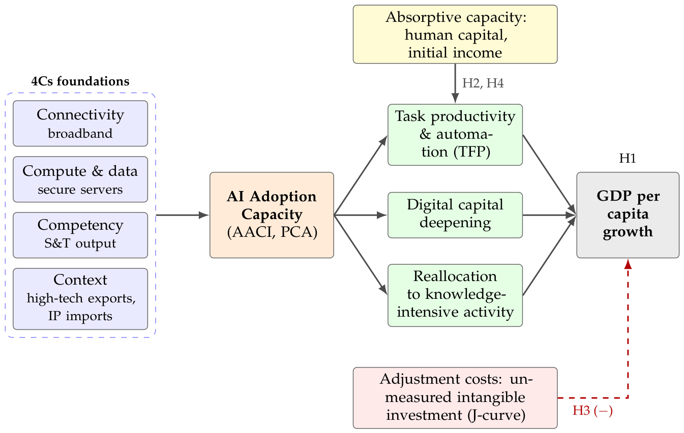
Figure 2.
AI Adoption Capacity Index by region, 2010–2023 (unweighted regional means; pooled standard-deviation units).
Figure 2.
AI Adoption Capacity Index by region, 2010–2023 (unweighted regional means; pooled standard-deviation units).
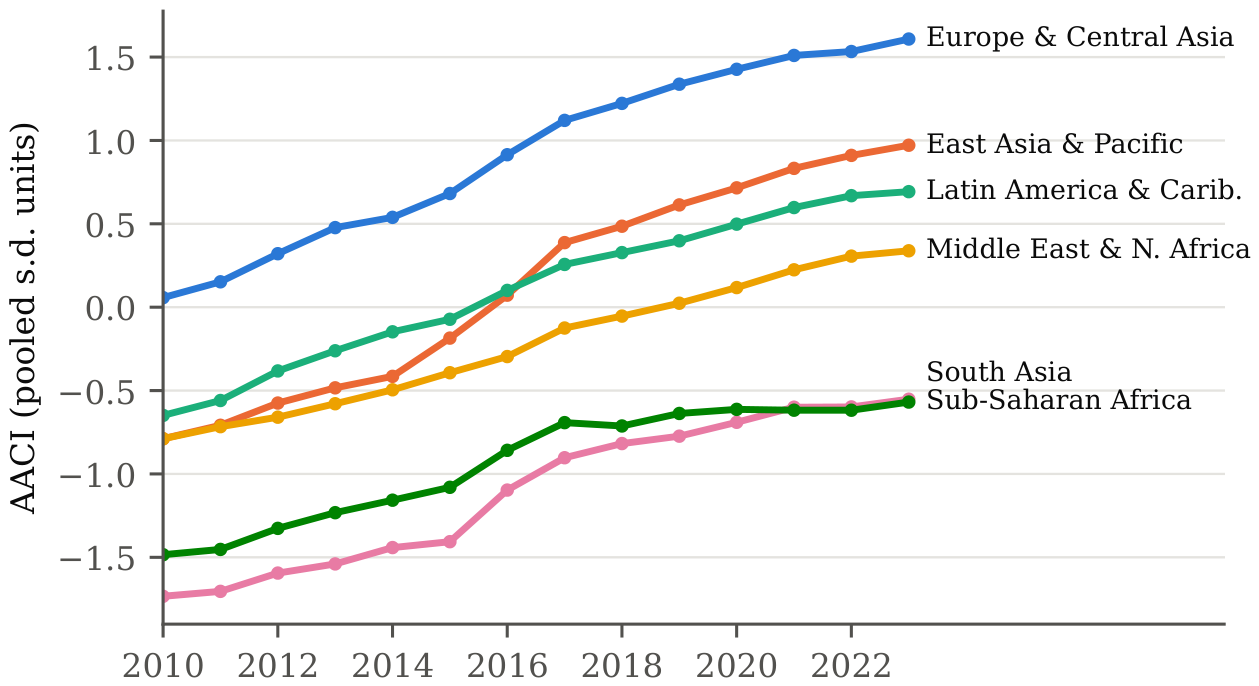
Figure 3.
Marginal effect of on GDP per capita growth by tertiary enrolment (Table 7, column 1), with 95% Driscoll–Kraay confidence band. Rug marks show the sample distribution of enrolment.
Figure 3.
Marginal effect of on GDP per capita growth by tertiary enrolment (Table 7, column 1), with 95% Driscoll–Kraay confidence band. Rug marks show the sample distribution of enrolment.
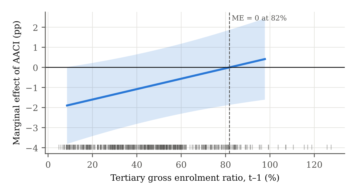
Figure 4.
coefficients across specifications, estimators and outcomes, with 95% confidence intervals. Blue: fixed effects with GDP per capita growth; green: alternative outcomes (2011–2019); orange: system GMM.
Figure 4.
coefficients across specifications, estimators and outcomes, with 95% confidence intervals. Blue: fixed effects with GDP per capita growth; green: alternative outcomes (2011–2019); orange: system GMM.
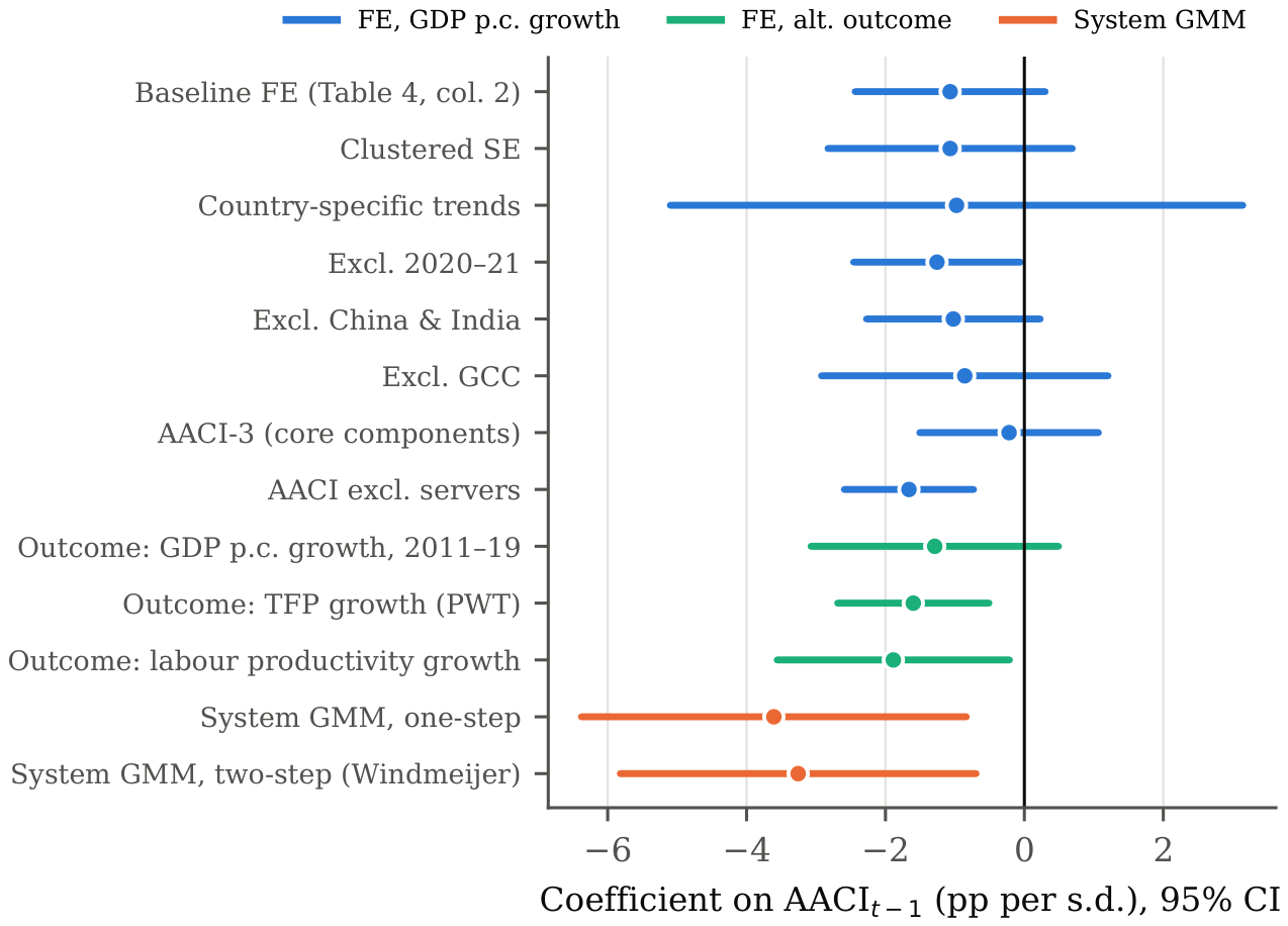
Figure 5.
Medium-run relationship: change in mean AACI against change in mean GDP per capita growth, 2018–23 vs. 2011–16 (bivariate fit shown; the regression with controls is reported in Table 8, panel D).
Figure 5.
Medium-run relationship: change in mean AACI against change in mean GDP per capita growth, 2018–23 vs. 2011–16 (bivariate fit shown; the regression with controls is reported in Table 8, panel D).
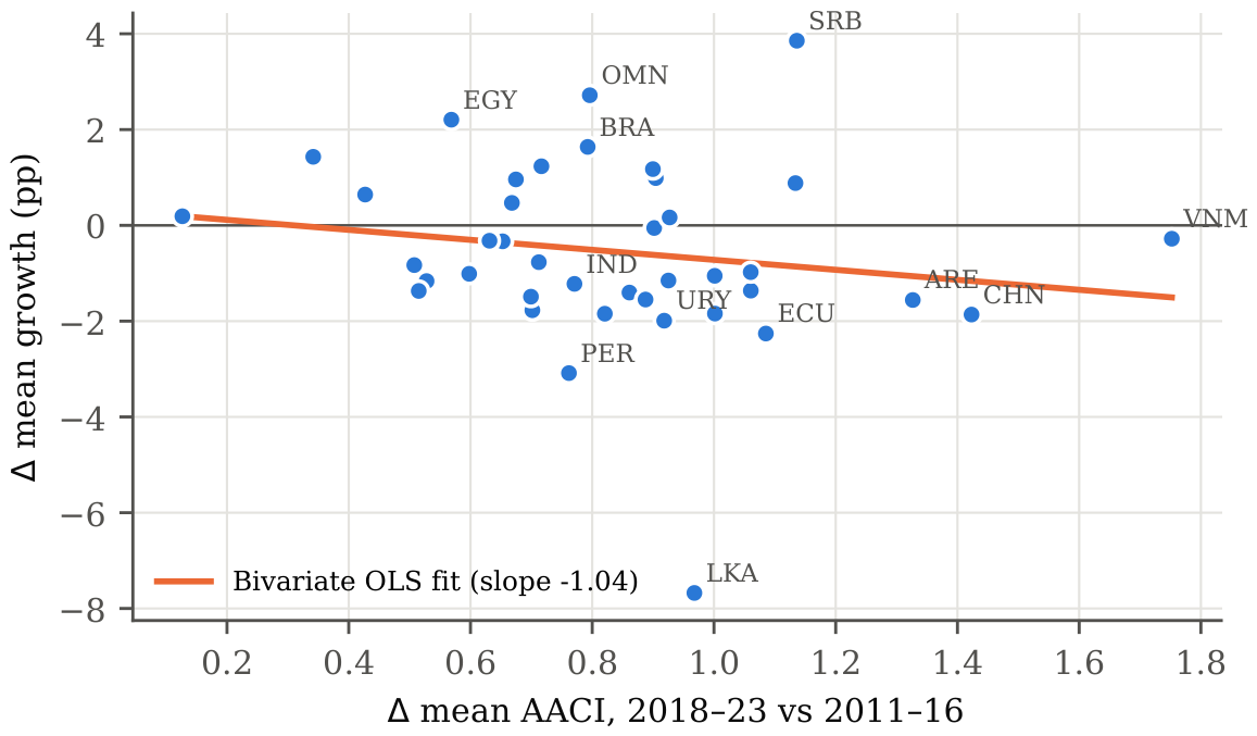
Figure 6.
Leave-one-country-out estimates of the baseline coefficient (Table 5, column 2), with 95% confidence intervals.
Figure 6.
Leave-one-country-out estimates of the baseline coefficient (Table 5, column 2), with 95% confidence intervals.
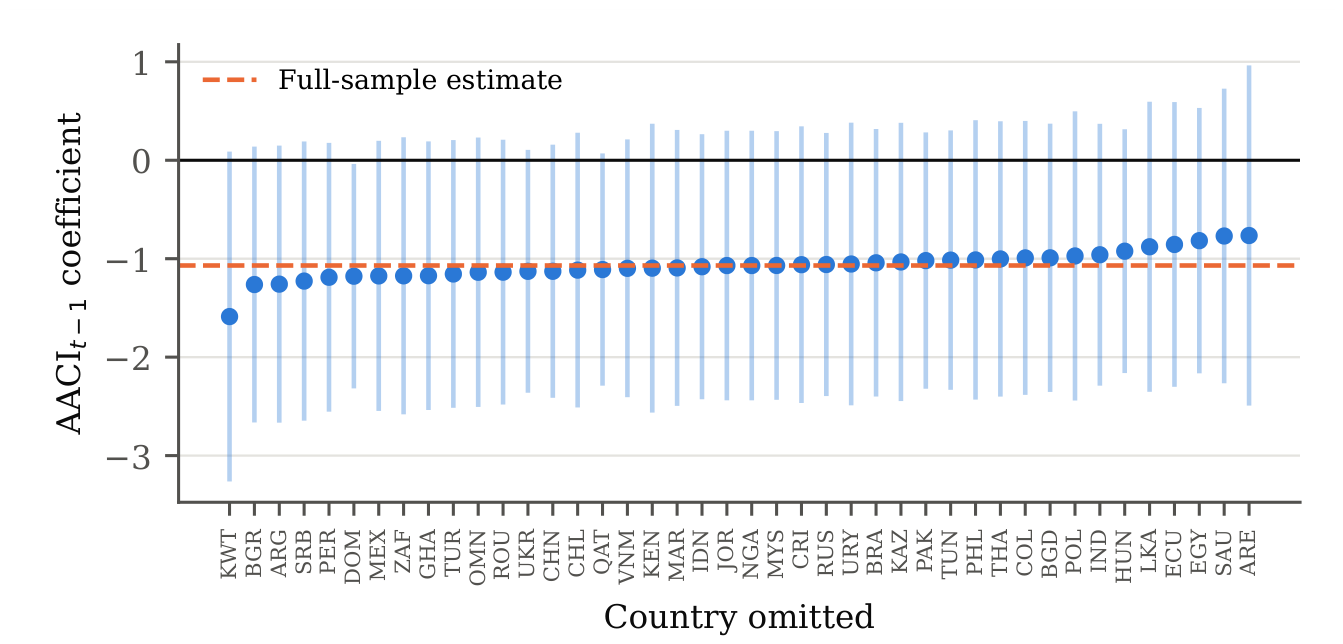
Table 1.
Synthesis of selected evidence on AI and growth.
| Study | Sample | Approach | Main finding |
| Acemoglu [1] | US | Task-based calibration | TFP gain ≈0.7% over 10 years |
| Aghion & Bunel [2] | US | Alternative aggregation | Larger gains under fast diffusion |
| Cazzaniga et al. [4] | 174 countries | Exposure & preparedness index | AEs more exposed and better prepared |
| Cerutti et al. [5] | Global | Multi-sector model | Gains skewed towards AEs |
| Gambacorta et al. [6] | 56 economies | Rajan–Zingales | Knowledge-intensive sectors gain; EMs benefit less |
| World Bank [8] | LMICs | 4Cs diagnostic | Foundations (4Cs) are binding |
| Lu [12] | Global panel | FE, GMM, AI patents | Positive long-run growth effect |
| Ho & Giwa [11] | 194 studies | Systematic review | Evidence fragmented; EMs under-studied |
| Brynjolfsson et al. [19] | US | Growth accounting | Intangibles create a productivity J-curve |
Table 2.
Variables, definitions and sources.
| Variable | Definition | Source (code) |
| Outcomes | ||
| Growth | Real GDP per capita growth, % | WDI (NY.GDP.PCAP.KD.ZG) |
| TFP growth | TFP at constant national prices | PWT 10.01 (rtfpna) |
| Labour productivity | (real GDP / persons employed) | PWT 10.01 |
| AACI components (4Cs) | ||
| Connectivity | Fixed broadband subscriptions per 100 people | WDI (IT.NET.BBND.P2) |
| Compute & data | secure internet servers per million) | WDI (IT.NET.SECR.P6) |
| Competency | ln(S&T journal articles per million people) | WDI (IP.JRN.ARTC.SC) |
| Context (production) | High-technology exports, % of manufactured exports | WDI (TX.VAL.TECH.MF.ZS) |
| Context (absorption) | IP charges paid, % of GDP) | WDI (BM.GSR.ROYL.CD) |
| Controls and moderators | ||
| Initial income | ln real GDP p.c. (2010 PPP $), | WDI |
| Investment | Gross capital formation, % GDP | WDI (NE.GDI.TOTL.ZS) |
| Population growth | Annual % | WDI (SP.POP.GROW) |
| Trade | ln(exports + imports, % GDP) | WDI |
| Inflation | , CPI (deflator if missing) | WDI (FP.CPI.TOTL.ZG) |
| FDI | Net inflows, % GDP (winsorised 1/99) | WDI (BX.KLT.DINV.CD.WD) |
| Human capital | Tertiary gross enrolment ratio, | WDI (SE.TER.ENRR) |
| Validation | ||
| AI patents | AI patent families by national office, priority years 2015–19 | CSET/1790 [13] |
Table 3.
Principal component loadings of the AACI (pooled 2010–2023).
| Pillar (4Cs) | Component | PC1 loading |
| Connectivity | Fixed broadband subscriptions (per 100) | 0.518 |
| Compute & data | Secure internet servers (log, per million) | 0.513 |
| Competency | S&T journal articles (log, per million) | 0.485 |
| Context | High-tech exports (% of manuf. exports) | 0.190 |
| Context | IP charges paid (log, % of GDP) | 0.445 |
| Variance explained by PC1 | 56.1% | |
Table 4.
Descriptive statistics, 42 emerging economies, 2011–2023.
| Variable | Obs. | Mean | S.D. | Min | Max |
| GDP per capita growth (%) | 546 | 1.99 | 4.05 | -22.75 | 15.45 |
| AACI (standardised) | 546 | 0.06 | 0.99 | -2.39 | 2.34 |
| Fixed broadband (per 100) | 543 | 11.97 | 9.58 | 0.01 | 44.73 |
| Secure servers (per million) | 546 | 2,985.9 | 8,062.5 | 0.5 | 57,819.6 |
| S&T articles (count) | 546 | 25,369.8 | 89,789.8 | 19.4 | 932,711.9 |
| High-tech exports (% manuf.) | 507 | 11.47 | 13.04 | 0.00 | 67.05 |
| IP charges paid (% GDP) | 465 | 0.31 | 0.27 | 0.01 | 1.60 |
| Log real GDP p.c. (2010 PPP $) | 546 | 9.61 | 0.81 | 7.90 | 12.05 |
| Gross capital formation (% GDP) | 520 | 24.35 | 6.84 | 8.21 | 49.49 |
| Population growth (%) | 546 | 1.22 | 1.92 | -10.93 | 14.23 |
| Trade (% GDP) | 520 | 74.12 | 37.88 | 22.49 | 199.04 |
| Inflation (%) | 546 | 6.65 | 9.98 | -2.54 | 133.49 |
| FDI inflows (% GDP) | 546 | 2.87 | 6.45 | -40.11 | 105.64 |
| Tertiary enrolment (gross %) | 525 | 47.59 | 23.72 | 5.75 | 127.58 |
| TFP growth (%, PWT, 2011–19) | 324 | -0.26 | 2.43 | -12.96 | 5.79 |
Notes: Sources: World Development Indicators (July 2026 vintage), Penn World Table 10.01. Component series are shown in natural units; the AACI uses their transformed values (Table 2).
Table 5.
Baseline two-way fixed-effects estimates. Dependent variable: real GDP per capita growth (%), 2011–2023.
Table 5.
Baseline two-way fixed-effects estimates. Dependent variable: real GDP per capita growth (%), 2011–2023.
| (1) | (2) | (3) | (4) | (5) | |
| Parsimonious | + Controls | Contemp. AACI | + Country trends | Excl. 2020–21 | |
| a | |||||
| Investment (% GDP) | |||||
| Population growth | |||||
| ln Trade (% GDP) | |||||
| ln(1+inflation) | |||||
| FDI inflows (% GDP) | |||||
| Country FE | Yes | Yes | Yes | Yes | Yes |
| Year FE | Yes | Yes | Yes | Yes | Yes |
| Country-specific trends | No | No | No | Yes | No |
| Observations | 546 | 520 | 520 | 520 | 440 |
| Countries | 42 | 40 | 40 | 40 | 40 |
| Within | 0.043 | 0.180 | 0.176 | 0.412 | 0.164 |
Notes: Driscoll–Kraay standard errors (Bartlett kernel, 2 lags) in parentheses, robust to heteroskedasticity, serial correlation and cross-sectional dependence. AACI is standardised (mean 0, s.d. 1), so coefficients give the percentage-point change in growth per one-standard-deviation increase. aColumn (3) uses contemporaneous AACIt . Columns (2)–(5) lose Jordan and Nigeria for lack of investment and trade data. *** p < 0.01, ** p < 0.05, * p < 0.1.
Table 6.
Addressing endogeneity: dynamic-panel GMM and fixed-effects IV estimates.
| (1) | (2) | (3) | (4) | (5) | (6) | |
| Sys-GMM | Sys-GMM | Sys-GMM | Diff-GMM | FE-IV | FE-IV | |
| one-step | two-step | two-step | one-step | peer AACI | peer AACI | |
| lags 2–3 | lags 2–3 | lags 2–4 | lags 2–3 | + reg. growth | ||
| () | ||||||
| Controls (exogenous) | Yes | Yes | Yes | Yes | Yes | Yes |
| Year effects | Yes | Yes | Yes | Yes | Yes | Yes |
| Instruments | 23 | 23 | 25 | 20 | – | – |
| AR(1) p-value | 0.022 | 0.028 | 0.026 | 0.072 | – | – |
| AR(2) p-value | 0.257 | 0.257 | 0.276 | 0.430 | – | – |
| Hansen Jp-value | 0.042 | 0.042 | 0.062 | 0.869 | – | – |
| First-stage F (excl. instr.) | – | – | – | – | 0.94 | 0.98 |
| Countries | 40 | 40 | 40 | 40 | 40 | 40 |
| Observations | 440 | 440 | 440 | 440 | 520 | 520 |
Notes: Columns (1)–(4): dependent variable 100 ln yit , so the AACI coefficient is directly comparable to the growth regressions (percentage points) and ρ − 1 is the annual convergence rate. ln yt−1 and AACIt−1 are treated as endogenous with collapsed instruments (Roodman, 2009); controls and year dummies are IV-style instruments. Column (1) reports one-step cluster-robust SE; (2)–(3) report two-step SE with the Windmeijer (2005) correction. Observations count first-differenced equations. Columns (5)–(6): two-way FE-2SLS; AACIt−1 instrumented by the leave-one-out regional mean AACIt−1; column (6) also controls for leave-one-out regional mean growth. Country-clustered SE. *** p < 0.01, ** p < 0.05, * p < 0.1.
Table 7.
Heterogeneity: complementarities, initial conditions, nonlinearity and regions.
| Panel A. Interactions (two-way FE, full control set) | ||||
| (1) | (2) | (3) | (4) | |
| Human capital | Low initial income | Low initial AACI | Quadratic | |
| (c.) | ||||
| Tertiary (c.) | ||||
| below-median | ||||
| below-median | ||||
| Observations | 510 | 520 | 520 | 520 |
| Countries | 40 | 40 | 40 | 40 |
| Panel B. Regional sub-samples: coefficient on | ||||
| East Asia & Pacific | , countries | |||
| South Asia | , countries | |||
| Latin America & Caribbean | , countries | |||
| Europe & Central Asia | , countries | |||
| Middle East & North Africa | , countries | |||
| Sub-Saharan Africa | , countries | |||
| Excluding China and India | , countries | |||
| Excluding GCC economies | , countries | |||
Notes: All regressions include country and year FE, ln yt−1 and the controls of Table 5; Driscoll–Kraay SE in parentheses. Tertiary enrolment is centred (c.) at its sample mean. In Panel B the coefficient is in the first numeric column and its SE in the second. Regional estimates rest on 3–10 countries and are indicative only. *** p < 0.01, ** p < 0.05, * p < 0.1.
Table 8.
Robustness: alternative measures, outcomes, timing and inference.
| Coefficient | SE | Obs. | Countries | |
| A. Alternative AI-adoption measures (outcome: GDP p.c. growth) | ||||
| AACI-3 (broadband, servers, articles) | 520 | 40 | ||
| AACI excluding secure servers | 520 | 40 | ||
| Fixed broadband only | 520 | 40 | ||
| Secure servers only | 520 | 40 | ||
| S&T articles only | 520 | 40 | ||
| High-tech exports only | 497 | 39 | ||
| IP charges paid only | 446 | 37 | ||
| B. Alternative outcomes, 2011–2019 (PWT 10.01 window) | ||||
| GDP p.c. growth (same window) | 360 | 40 | ||
| TFP growth ( rtfpna ) | 306 | 34 | ||
| Labour productivity growth | 360 | 40 | ||
| C. Timing, placebo and reverse causality | ||||
| , with lead included | 480 | 40 | ||
| Lead (placebo) | 480 | 40 | ||
| Reverse: on | 546 | 42 | ||
| Distributed lag: | 440 | 40 | ||
| 440 | 40 | |||
| 440 | 40 | |||
| Cumulative (sum of lags 1–3) | 440 | 40 | ||
| D. Medium run: long difference (2018–23 vs 2011–16 means), cross-section | ||||
| AACI (controls: , investment) | 40 | 40 | ||
Notes: Panels A–C: two-way FE with and the full control set (except the reverse-causality row, which conditions on only); Driscoll–Kraay SE. Single-component measures are standardised. Panel D: OLS with HC1 SE. *** , , .
Disclaimer/Publisher’s Note: The statements, opinions and data contained in all publications are solely those of the individual author(s) and contributor(s) and not of MDPI and/or the editor(s). MDPI and/or the editor(s) disclaim responsibility for any injury to people or property resulting from any ideas, methods, instructions or products referred to in the content. |
© 2026 by the authors. Licensee MDPI, Basel, Switzerland. This article is an open access article distributed under the terms and conditions of the Creative Commons Attribution (CC BY) license (http://creativecommons.org/licenses/by/4.0/).
Copyright: This open access article is published under a Creative Commons CC BY 4.0 license, which permit the free download, distribution, and reuse, provided that the author and preprint are cited in any reuse.