Submitted:
17 November 2025
Posted:
17 November 2025
You are already at the latest version
Abstract
This paper introduces new methods of a mathematical framework for analyzing and reducing harmonic distortion in small-signal DC–DC converters. Traditional methods often depend on large passive components or trial-and-error tuning, which can be costly and lack precise predictive power. In contrast, this work defines a harmonic reduction coefficient (Δ), derived analytically from small-signal transfer functions, serving as a design tool to quantify and minimize harmonic content. Closed-form formulas for the resonant frequency and Δ are developed for Buck, Boost, and Buck–Boost converters operating in continuous conduction mode (CCM). The proposed approach enables the optimal selection of passive components to effectively suppress second-harmonic distortion, eliminating the need for additional filtering hardware. Simulations confirm the theoretical findings, showing significant improvements in total harmonic distortion (THD). Overall, the Δ-based design method offers a practical and versatile tool for enhancing converter performance in sensitive applications, including radar systems, audio equipment, and renewable energy interfaces.
Keywords:
DC–DC converters
; harmonic distortion
; small-signal modeling
; perturbation theory
; total harmonic distortion (THD)
; harmonic reduction coefficient
1. Introduction
Switching DC–DC converters are widely used in power supplies, renewable energy systems, communication electronics, and defense applications. Despite their advantages in efficiency and compactness, these converters inherently generate harmonic distortion due to their switching operation and nonlinear dynamics. In small-signal operation, the output voltage typically exhibits an AC ripple superimposed on the DC level, with significant contributions from low-order harmonics. Among these, the second harmonic is particularly problematic: it can induce oscillatory behavior in low-frequency systems, cause perceptible flicker effects in lighting, and introduce distortion in sensitive audio or radar equipment (Wang et al., 2023; Shen et al., 2024).
Traditional approaches to harmonic suppression rely on passive filtering, employing large inductors or high-capacitance components to attenuate ripple (Park et al., 2021). While effective, such methods increase system size, weight, and cost, often involving empirical tuning rather than predictive design. More advanced strategies include active compensation schemes (Zhang & Ruan, 2018; Li et al., 2024) and harmonic current reduction in PFC or resonant converter stages (Ruan et al., 2022a; Ruan et al., 2022b). Although these solutions can reduce distortion, they generally require additional circuitry or involve complex optimization processes.
Recent developments in modeling frameworks have focused on harmonic-state-space (HSS) and multifrequency small-signal approaches (Motwani et al., 2022; Mei et al., 2020; Li et al., 2022). These models provide powerful analysis tools but are mathematically intensive and less practical for straightforward component design. Other works have explored building-block state-space modeling (Herbst, 2019), advanced resonant modeling (Corti et al., 2025), and harmonic mitigation in rectifier and inverter front-ends (Du et al., 2021; Grosso et al., 2023). However, few offer closed-form, design-oriented metrics directly linking component values to harmonic attenuation.
This paper addresses this gap by introducing the concept of a harmonic reduction coefficient (Δ), derived from small-signal transfer functions using perturbation theory and separation-of-variables analysis. Unlike previous works, the proposed Δ-based framework directly quantifies the relationship between passive component values and harmonic suppression effectiveness. The main contributions are as follows:
1) A unified modeling framework for Buck, Boost, and Buck–Boost converters operating in CCM, extending earlier small-signal and resonant converter analyses (Yang et al., 1992; Tian et al., 2016; Vyapari, 2022).
2) A new design-oriented metric: the harmonic reduction coefficient Δ, enabling predictive suppression of low-order harmonics.
3) Closed-form analytical expressions for resonant frequency and Δ in major converter topologies.
4) Validation through MATLAB/Simulink simulation showing significant reduction of THD, complementing recent control-based suppression strategies (Escobar et al., 2021).
2. Theoretical Framework and Modeling
Harmonic suppression in converters has been studied from multiple perspectives. Passive filtering remains the most conventional solution (Park et al., 2021), though it is constrained by size and cost limitations. Active strategies, such as one-cycle control and harmonic current injection, have been successfully applied in single-phase inverters and DC-link converters (Zhang & Ruan, 2018; Li et al., 2024), while multi-stage architectures with resonant converters offer partial suppression of second-harmonic current (Ruan et al., 2022a; Ruan et al., 2022b).
On the modeling side, harmonic-state-space (HSS) techniques (Motwani et al., 2022; Mei et al., 2020; Li et al., 2022) and building-block small-signal approaches (Herbst, 2019) have deepened understanding of converter dynamics, but often at the expense of design tractability. Recent works on advanced resonant converter modeling (Corti et al., 2025; Tian et al., 2016) provide insights into harmonic propagation but lack a unified analytical metric for harmonic reduction. Reviews of multipulse rectifier and three-phase converter systems further highlight the importance of harmonics in large-scale applications (Du et al., 2021; Grosso et al., 2023).
In contrast, the present work develops a simplified yet rigorous mathematical framework that captures the essential harmonic behavior of Buck, Boost, and Buck–Boost converters. The proposed harmonic reduction coefficient (Δ) directly links circuit parameters to harmonic attenuation, filling the gap between detailed modeling and practical design guidelines.
Traditional approaches for characterizing the AC behavior of DC–DC converters often rely on detailed transfer function analysis, such as state-space averaging [1]. While accurate, many of these models are mathematically complex and cumbersome for routine engineering applications [2,4,5]. In contrast, the approach proposed herein emphasizes simplicity and analytical clarity, drawing on the methodology developed in this paper, which enables practical prediction of harmonic behavior with high accuracy.
The proposed mathematical framework is designed to be generalizable across various DC–DC converters and adaptable to custom design constraints.
However, the methods of large inductors or capacitors are not always cost-effective and often involve over-dimensioning. The core objective of this research is to derive analytically optimized component values that simultaneously meet system specifications and undesirable harmonics, particularly the second harmonics.
The underlying methodology employs perturbation theory in conjunction with a separation-of-variables approach. This framework divides circuit elements into two categories: fast-response elements (e.g., switches, diodes, and resistors) and slow-response elements (e.g., inductors and capacitors). Perturbations are then applied to the slow variables to derive a comprehensive transfer matrix. This matrix encapsulates the system’s small-signal behavior and serves as the foundation for calculating harmonic suppression characteristics.
This analytical technique is validated through implementation in MATLAB and Simulink. The simulation results confirm that the derived component values not only suppress the second harmonic effectively but also minimize total harmonic distortion (THD) without resorting to excessive filtering.
This method partitions circuit variables into:
- **Fast-response**: Resistors, diodes
- **Slow-response**: Filter inductors, capacitors(as output voltage), input voltage, duty cycle switch.
The slow response variables (as mentioned earlier and oscillating components) will be the and , this paper will use as and as for simplicity.
Perturbation theory is applied to slow-response variables:
Traditional approaches for characterizing the AC behavior of DC–DC converters often rely on detailed transfer function analysis, such as state-space averaging [1]. While accurate, many of these models are mathematically complex and cumbersome for routine engineering applications [2,4,5]. In contrast, the approach proposed herein emphasizes simplicity and analytical clarity, drawing on the methodology developed in this paper, which enables practical prediction of harmonic behavior with high accuracy.
The proposed mathematical framework is designed to be generalizable across various DC–DC converters and adaptable to custom design constraints.
This yields the small-signal CCM transfer matrix:
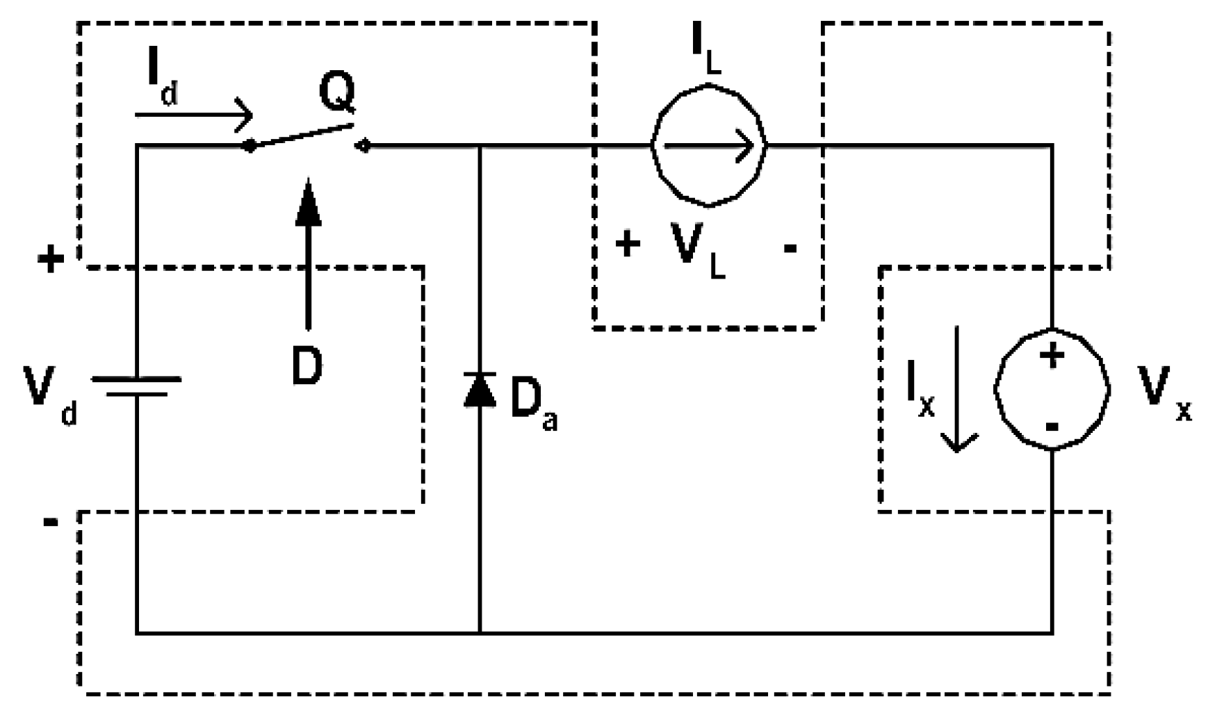
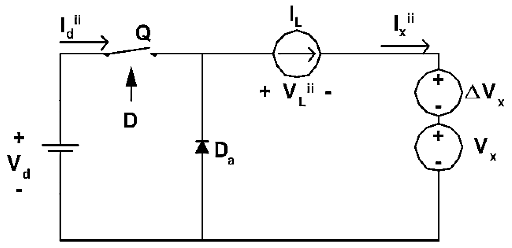
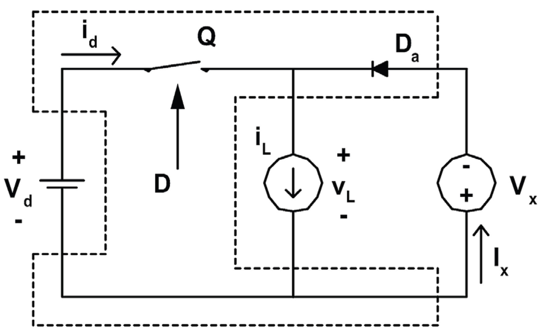
And a general small signal model as shown in Figure 1
This approach enables explicit derivation of matrix elements per converter topology, following the formalism established by Orugani [3] and Keong [18].
The averaged small signal equivalent circuit is used to relate the variations in output voltage to changes in input voltage and duty cycle. Based on Kirchhoff’s current and voltage laws, the following relationships for a simplified converter model can be written as:
Substituting into the general transfer matrix form Equation (2), the complete small-signal transfer function can be obtained:
Solving for the output to input voltage small-signal transfer function is:
This mathematical formulation forms the basis for evaluating harmonic distortion characteristics and designing component values for suppression of second harmonic effects in the following section, as for simplicity, we will express the output to input voltage perturbation as a frequency response function due its dependence on a frequency.
3. Harmonic Analysis of Converter Topologies
3.1. Buck Converter Small-Signal Analysis in CCM
The Buck converter, operating in continuous conduction mode (CCM), serves as the foundational case for small-signal analysis. Utilizing state averaging and perturbation theory, the transfer matrix is derived by analyzing the dynamic behavior of both slow and fast variables. The circuit is decomposed into two parts: an averaged equivalent model and a fast-dynamic circuit. Perturbations are introduced for input voltage, inductor current, duty cycle, and output voltage. These perturbations are systematically applied to formulate the full transfer matrix. This matrix captures the system’s dynamic behavior around the nominal operating point and is foundational for analyzing frequency-dependent gain and harmonic suppression.
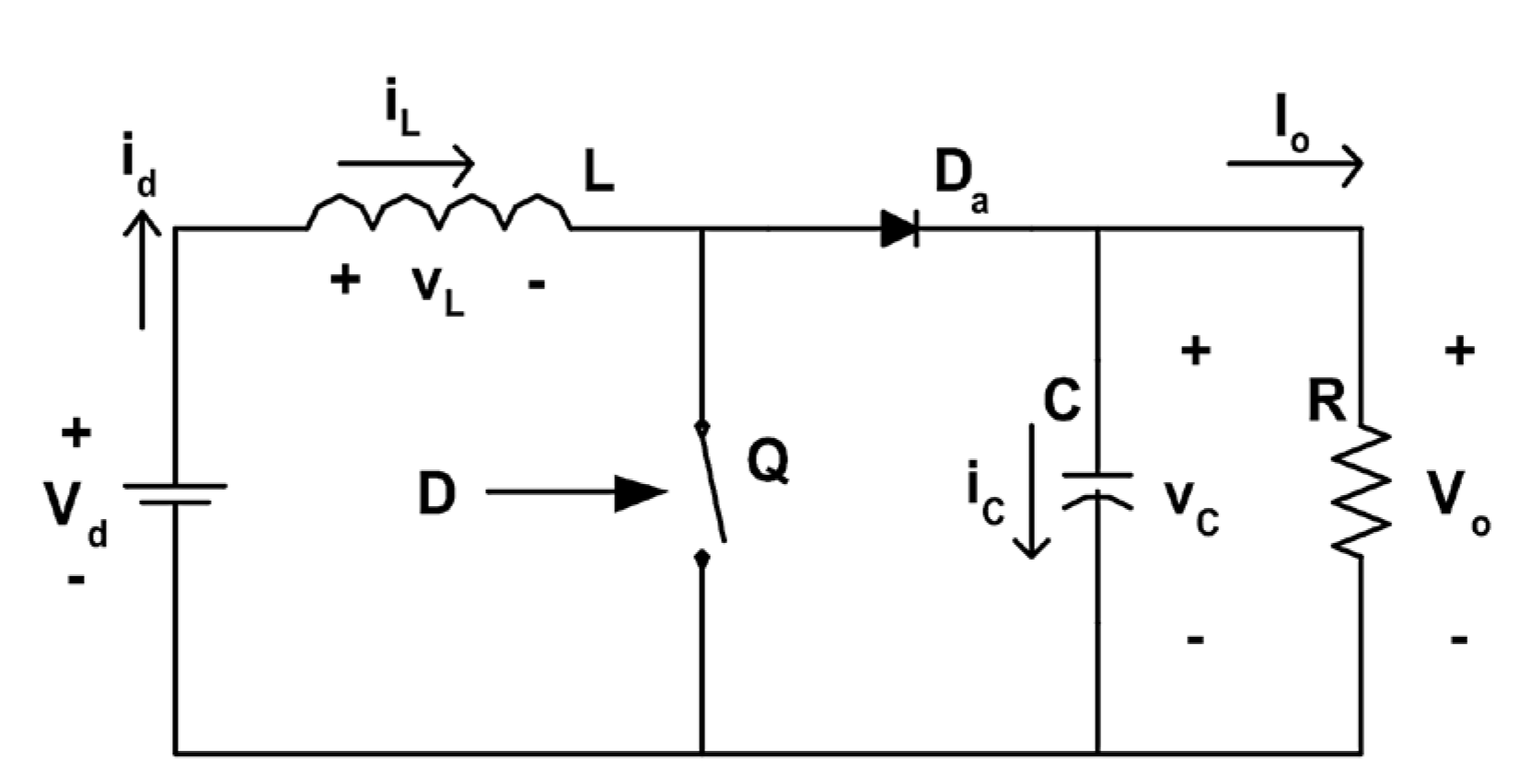
Classical converter in Figure 3. As follows:
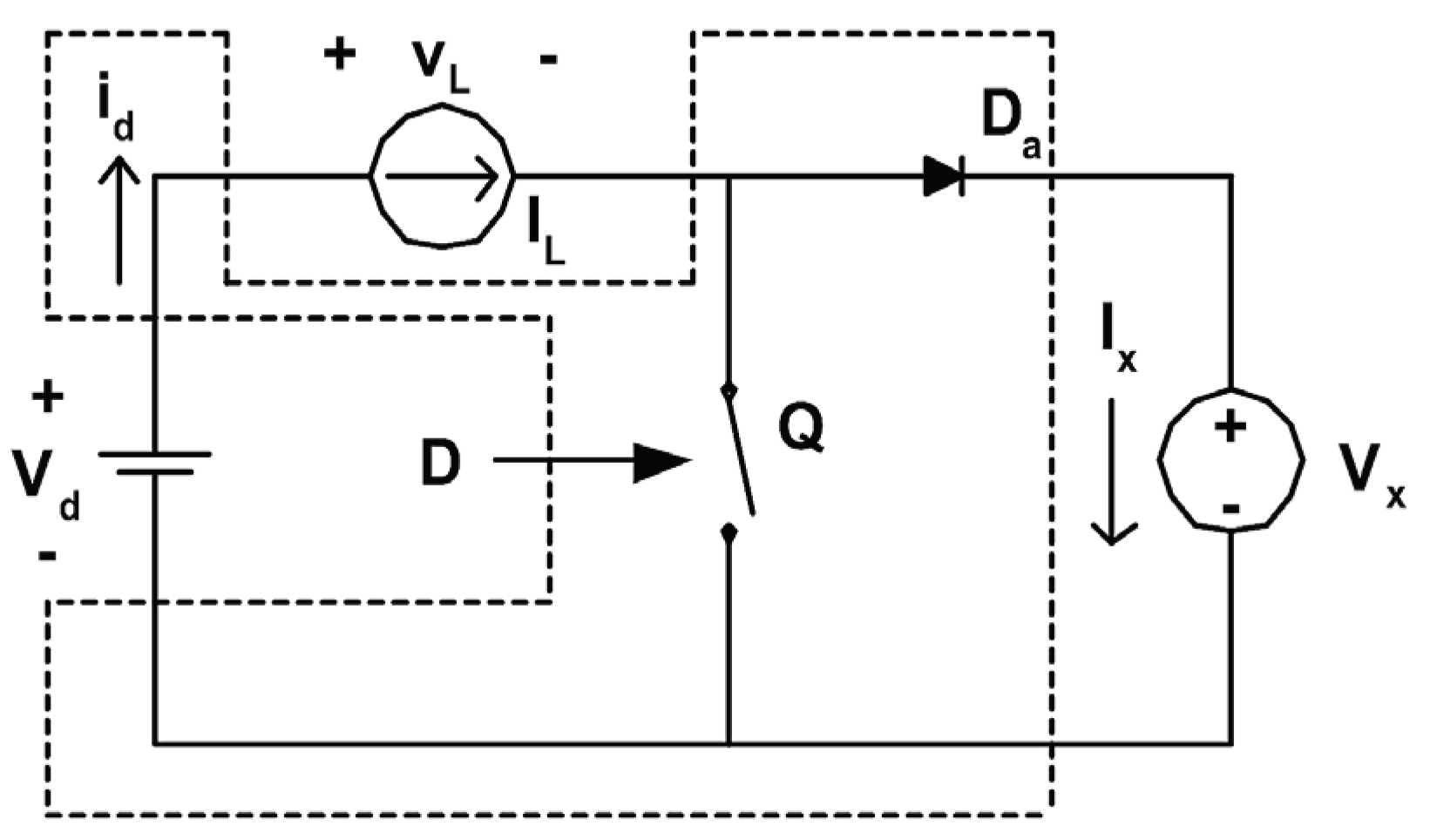
An equivalent fast dynamic model is:
Figure 4.
Fast dynamic Buck model. A presentation of perturbed variables of the circuit.
State variables , , are obtained through averaging
Perturbation analysis yields:
Perturbation of an Input voltage.
Figure 5.
Input voltage perturbation. A perturbation of an input voltage variable and the calculated values as represented in a set of Equations (10).
Figure 5.
Input voltage perturbation. A perturbation of an input voltage variable and the calculated values as represented in a set of Equations (10).
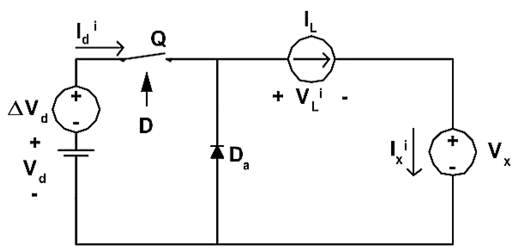
Figure 6.
Inductor current perturbation. A perturbation of an inductor variable and the calculated values as represented in a set of Equations (11).
Figure 6.
Inductor current perturbation. A perturbation of an inductor variable and the calculated values as represented in a set of Equations (11).
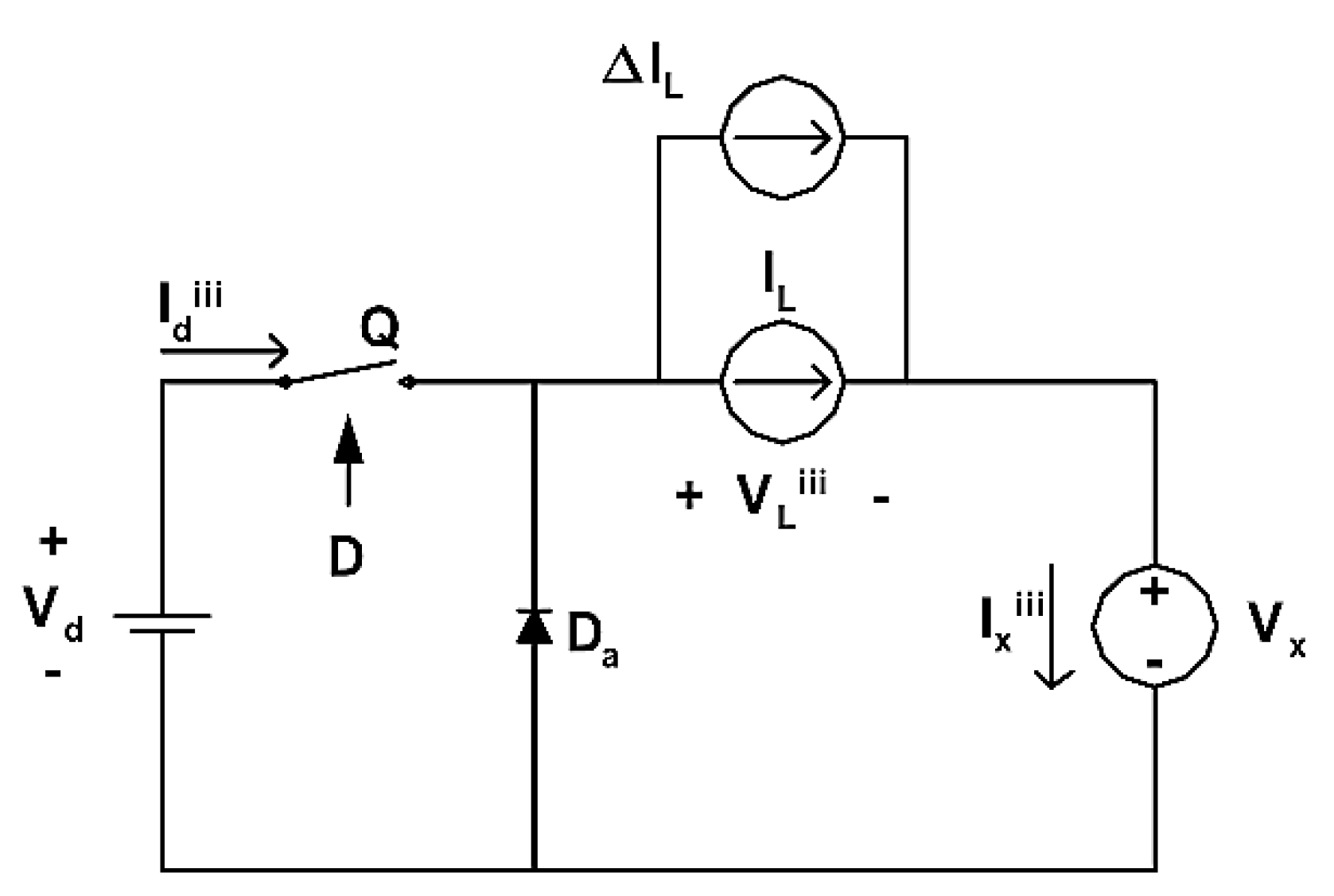
Figure 7.
Duty cycle ratio perturbation. A perturbation of a duty cycle variable and the calculated values as represented in a set of Equations (12).
Figure 7.
Duty cycle ratio perturbation. A perturbation of a duty cycle variable and the calculated values as represented in a set of Equations (12).
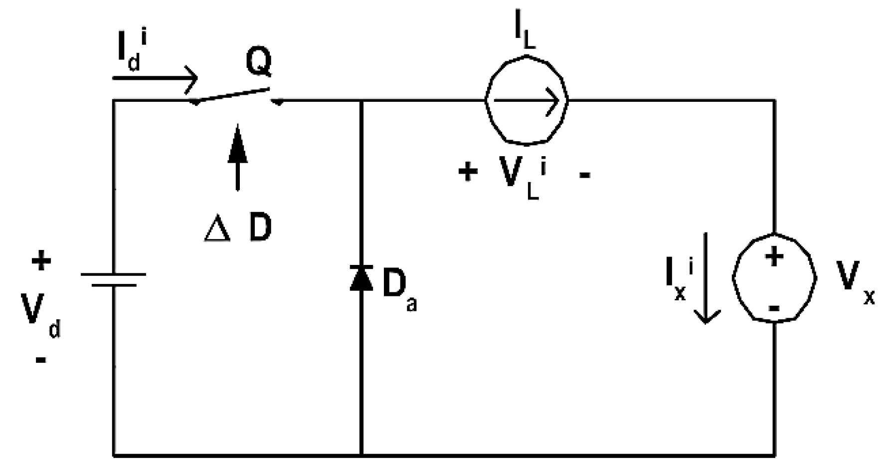
Figure 8.
Output voltage perturbation. A perturbation of an output voltage variable and the calculated values as represented in a set of Equations (13).
Figure 8.
Output voltage perturbation. A perturbation of an output voltage variable and the calculated values as represented in a set of Equations (13).
As presented by Equations (10), (11), (12), and (13), the final composite transfer matrix is:
Using the transfer function derived earlier, Equation (6), and substituting the matrix elements from the Buck converter Equation (14), the simplified transfer function becomes:
To analyze the magnitude of the transfer function in the frequency domain, as was mentioned earlier, the frequency response function will be then:
The maximum value of the function occurs at the resonant angular frequency given by:
At this frequency, the transfer function's magnitude reaches:
3.2. Boost Converter Small-Signal Analysis in CCM
As was performed in the previous section, the same principle will be implemented here.
State variables , , are obtained through averaging
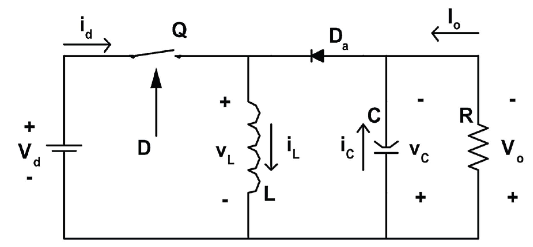
Figure 9.
Classical Boost converter topology. The usual and well-known Boost converter topology for a voltage increase in a DC-DC converter.
Figure 9.
Classical Boost converter topology. The usual and well-known Boost converter topology for a voltage increase in a DC-DC converter.
And a fast dynamic model is:
Figure 10.
Fast dynamic Boost model. A presentation of perturbed variables of the circuit.
Which yields the following results:
Perturbation analysis yields:
ΔId= ΔIL
ΔIx= (1-D)ΔIL -ILΔD
ΔVL=ΔVd -(1-D)ΔVx+Vx ΔD
The composite transfer matrix is:
Using Equations (6) and (23), the transfer function will be:
And the magnitude in the frequency domain is:
The resonant frequency at which this function reaches its peak is given by:
At this frequency, the peak value of the transfer function is:
3.3. Buck-Boost Converter Small-Signal Analysis in CCM
As was performed in the previous section, the same principle will be implemented here.
State variables , , are obtained through averaging
Figure 11.
Classical Buck-Boost converter topology. The usual and well-known Buck-Boost converter topology for a voltage increasing/decreasing of DC-DC converter.
Figure 11.
Classical Buck-Boost converter topology. The usual and well-known Buck-Boost converter topology for a voltage increasing/decreasing of DC-DC converter.
And a fast dynamic model is:
Figure 12.
Fast dynamic Buck-Boost model. A presentation of perturbed variables of the circuit.
Which yields the following results:
Perturbation analysis yields:
ΔId= ΔIL
ΔIx= (1-D)ΔIL -ILΔD
ΔVL=ΔVd -(1-D)ΔVx+Vx ΔD
The composite transfer matrix is:
Using Equation (6), (24), the transfer function will be:
And the magnitude in the frequency domain is:
The resonant frequency at which this function reaches its peak is given by:
At this frequency, the peak value of the transfer function is:
4. Design Examples and Simulation Validation
4.1. Buck Converter Harmonic Analysis
As a practical validation of the theory, consider a converter with the following parameters and under the CCM conditions for
:
Design example:
Substituting these values into Equation (17), the resonant frequency is calculated as:
or the frequency as . This matches the peak in the MATLAB plot simulation in Figure 13.
The plot in Figure 13 shows the transfer function magnitude in decibels ( as a function of frequency, with the peak occurring at approximately 1100 Hz and
which is very consistent with the theory. At 50Hz (or 100Hz for the second harmonic), the gain is substantially lower, indicating limited attenuation.
As a Simulink simulation, consider a simple Buck converter circuit as an AC disturbed signal of applied to the DC working voltage of V=28V in Figure 14.
The input signal Figure is:
The FFT analyzes the THD of the voltage input and output transfer function.
The THD in both input and output voltage is the same and small, but it was obvious by examining Figure 13, Figure 14, Figure 15, Figure 16, Figure 17 and Figure 18, where the disturbed voltage is almost pure sign of 50Hz frequency (except switching frequency that induces a small harmonics), and parameters of the components have been chosen to satisfy peak frequency, which is very far from the working frequency (50Hz).
To effectively suppress the second harmonic, the design must shift the resonant (knee) frequency to be smaller than the target frequency (second harmonic frequency). This is accomplished by selecting new component values such that the knee frequency will be smaller than the second harmonic, enabling attenuation from the resonant frequency to the target frequency. The reduction coefficient Δ in decibels is defined by comparing the gain at the Target (second harmonic) frequency to the DC (ω=0) gain:
Given a desired suppression (e.g., 39.9 dB) and design parameters such as
The required capacitor value for a resonant frequency of 10Hz is calculated as
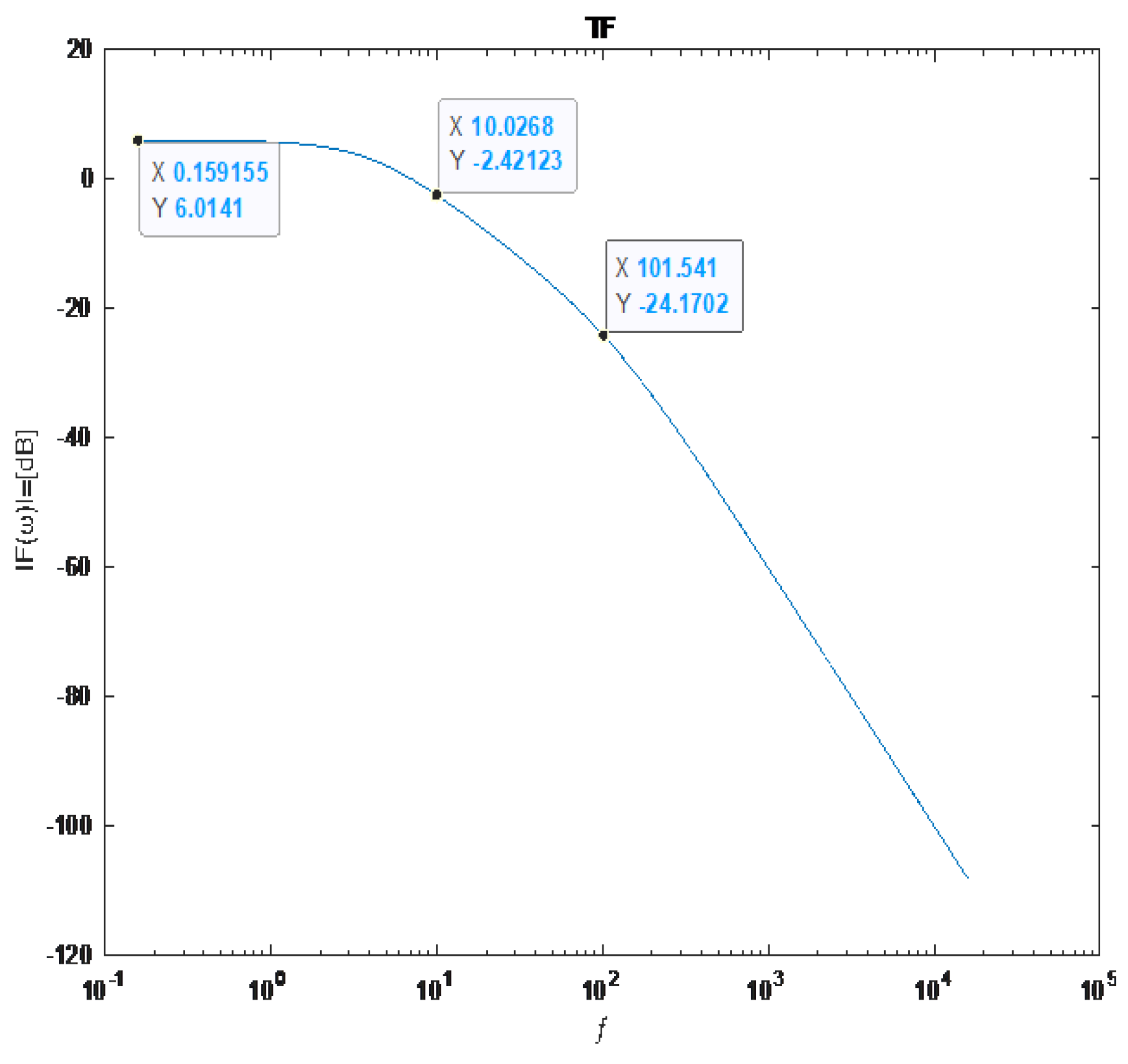
C1 = 12.64mF. Simulations confirm the theoretical prediction by showing the reduced gain at 10Hz to target a 100Hz frequency. As appears in the response plot in Figure 19
Figure 20.
Transfer function Plot as a dependence of frequency for L=20mH and.
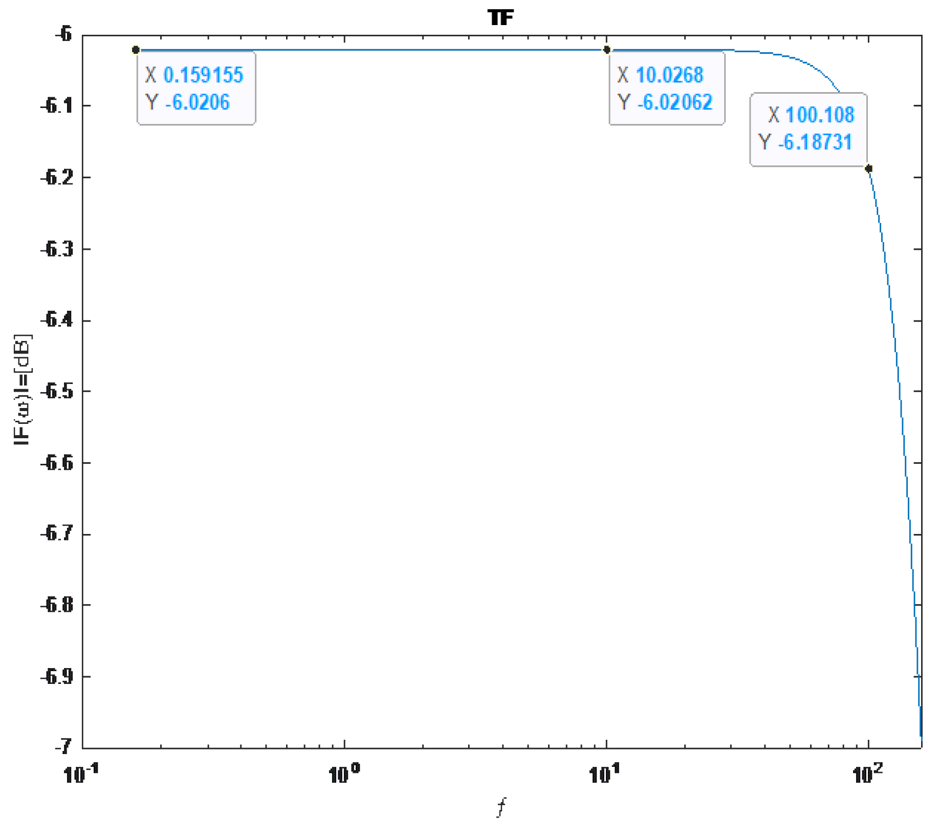
C=12.64mF as shown for the second harmonic at 100Hz, the transfer function has a value of -45dB, a reduction of 39.9 dB from a saturation line.
Alternatively, due to the nonlinearity of Equation (17), the same target frequency can also be achieved at but in this case, the reduction gain will have the value of
A MATLAB plot simulation of the second case is:
C= As shown for the second harmonic at 100Hz, the transfer function has a value of -6.18dB. A reduction of 0.16 dB from a saturation line.
Both conFigure urations represent the target angular frequency of but with different attenuation.
For the analysis, consider a realistic design with a full bridge rectifier and a capacitor filter of to reduce high ripple and the parameters as in the previous design (), although without the filter capacitor, we will get very high input harmonics, the output results of the harmonics will still be very satisfactory and highly reduced
Using the simulation structure (Figure 21), we can get results that characterize system behavior Figure 22, Figure 23, Figure 24, Figure 25, Figure 26 and Figure 27. The first design with and the reduction coefficient of
The FFT analysis will then be:
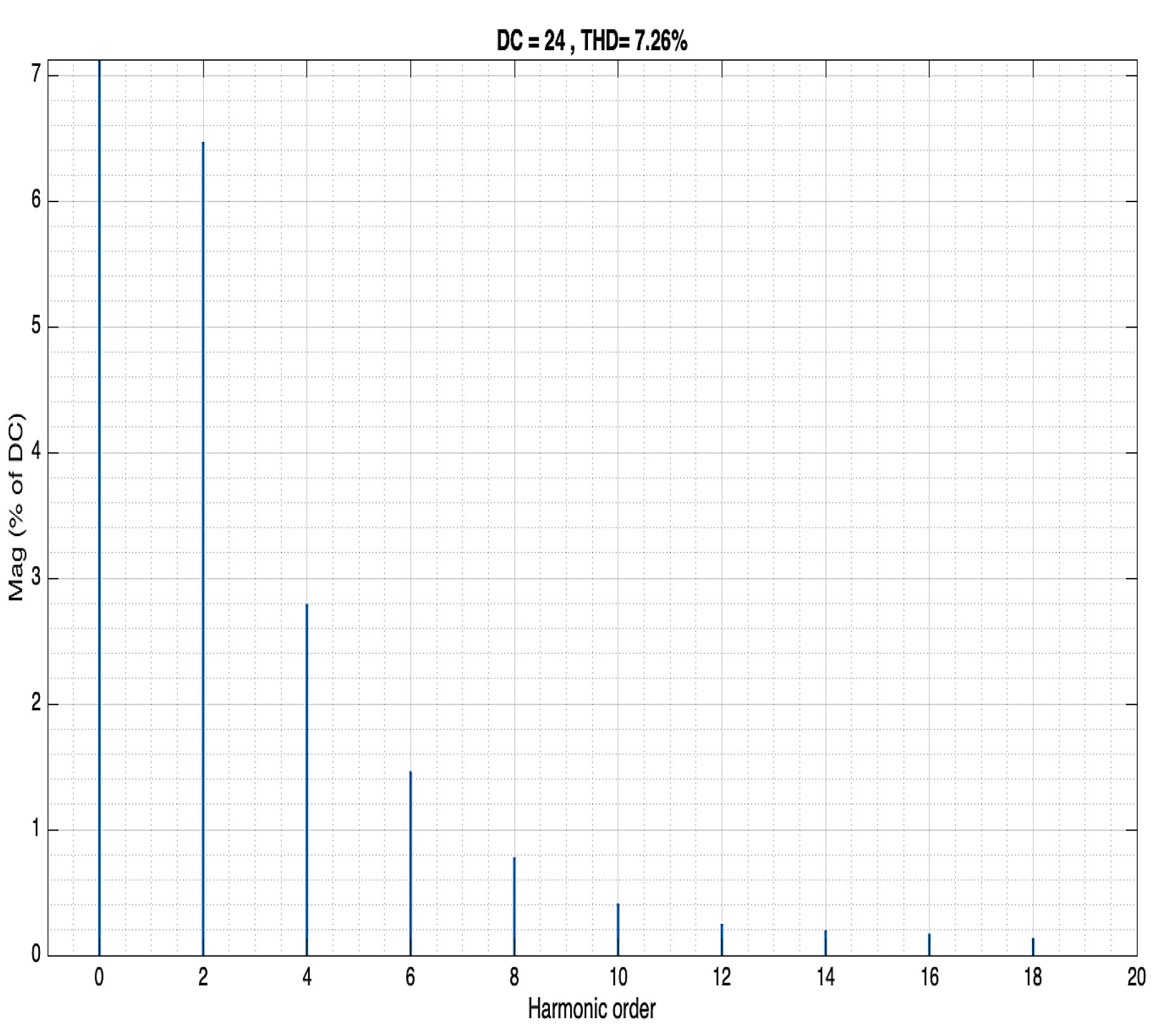
And for the second case design with
The presentation of the design with nominated customized component values was resolved mathematically by the reduction coefficient of the specific cost-effective design, which reduced THD.
The same methodological framework is applied to the Boost and Buck–Boost converters. The classical averaged Equations are derived for each topology, and the small-signal transfer matrix is constructed through the perturbation of key system variables. The derived transfer functions demonstrate topological dependence on passive component values and modulation parameters, such as duty cycle.
In both Boost and Buck–Boost cases, component sensitivity significantly influences the location and amplitude of resonance peaks, particularly near the system’s knee frequency. These peaks correspond to heightened harmonic content, especially at low-order harmonics such as the second harmonic.
4.2. Boost Converter Harmonic Analysis
To quantify harmonic suppression at a specific frequency, such as the second harmonic (typically 100Hz if the base is 50Hz), we define a reduction coefficient in decibels:
Note that the DC gain (saturation line) in Boost converter is
Design example:
To reduce the second harmonic, consider the following component values:
Input voltage:
Output voltage:
Duty cycle:
Load resistance:
Switching frequency:
Inductor: under CCM condition L
The aim of the suppression of which is suitable for a resonant frequency of 10Hz. By using Equation (38), the calculation of the required capacitor is:
Alternatively, the second choice of the capacitor by the same resonant frequency as calculated by Equation (26) is:
However, the harmonic suppression with is significantly weaker, as the MATLAB plot simulation shows for both cases, Figure 28 and Figure 29:
As indicated in Figure 29 and calculated by Equation (38), the reduction with the design is
For the Boost analysis, consider a model with a full bridge rectifier but without a filter capacitor (unnecessary due to the inductor filtering).
The input voltage in both cases will be considered the same due to an insignificant difference.
The FFT analysis will be:
With the aim of suppressing
4.3. Buck-Boost Converter Harmonic Analysis
As with previous converters, the reduction coefficient defines the suppression level compared to the saturation line at and at a specific frequency (second harmonic):
Design example:
To reduce the second harmonic, consider the following component values:
Input voltage:
Output voltage:
Duty cycle:
Load resistance:
Switching frequency:
Inductor: under CCM condition L To achieve a reduction coefficient which is once more suitable for ƒ=10Hz, the calculation of the required capacitor yields: and an alternative conFigure uration with the same target frequency but reduced attenuation yields .
And a reduced coefficient for is
The next Simulink results (Figure 35, Figure 36 and Figure 37) are shown when using Buck-Boost small signal model with a full bridge rectifier and a C=150μF filter to reduce the ripple:
As it was observed, the conFigure uration achieves deep second harmonic suppression while the produces limited attenuation despite having the same resonant frequency, which was determined by Equation (35), and the reduction coefficient of the Equation (39).
5. Discussion
The primary contribution of this work lies in the development and application of a general mathematical framework for suppressing harmonic distortion, primarily but not exclusively, in small-signal DC-DC converters. The approach is based on deriving and analyzing transfer functions using the separation of variables technique.
A key result is the formulation of the reduction coefficient Δ, which allows engineers to precisely estimate the amount of harmonic attenuation achievable at a specified (second harmonic) frequency and determine the resonant frequency as well. The reduction coefficient is dependent on system customized parameters and is unique to each converter topology.
An important observation is the transition of the resonant frequency from the real to the complex domain. When component values cause the expression under the square root in the resonant frequency Equations to become negative, the system exhibits no real knee frequency. Even in such cases, the reduction coefficient still predicts THD behavior accurately, demonstrating the robustness of the method.
As an example, consider a Boost converter with:
And a reduction coefficient of Δ=30dB
The required capacitor is but the corresponding frequency is imaginary ƒ=.
The simulation confirms that even without a real knee frequency, significant THD suppression is still achieved.
MATLAB plot simulation:
Figure 38.
Transfer function for Boost converter with components L=200mH and C2=64μF, attenuation of
Figure 38.
Transfer function for Boost converter with components L=200mH and C2=64μF, attenuation of
FFT analysis will be then:
Figure 39.
Input voltage as a function of harmonic order with components L=200mH and C2=64μF.
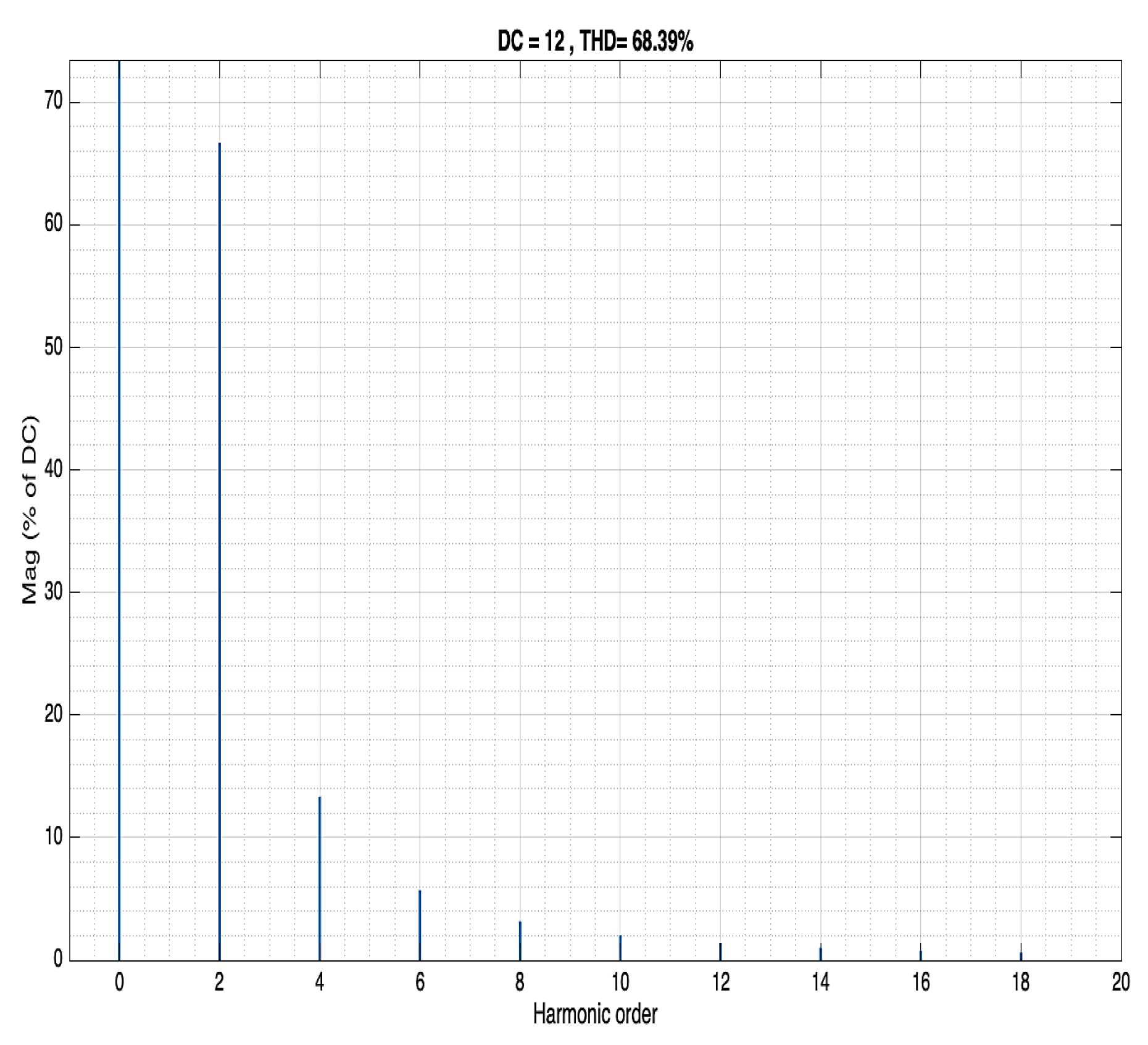
Figure 40.
Output voltage as a function of harmonic order with components L=200mH and C2=64μF, attenuation of
Figure 40.
Output voltage as a function of harmonic order with components L=200mH and C2=64μF, attenuation of
Several insights emerge from the study:
• The harmonic reduction coefficient serves as a reliable metric for guiding design trade-offs between harmonic suppression and component sizing.
• The saturation response of the system is topology-dependent: negative in Buck converters, positive in Boost converters, and variable in Buck–Boost conFigure urations based on the duty cycle, due to logarithmic dependence.
• The presence or absence of a knee frequency—and the sign of the second derivative of the transfer function—indicates whether there will be a knee frequency (positive second derivative) or absence of the knee frequency (negative second derivative).
These observations contribute to a deeper understanding of the physical behavior and design sensitivity of small-signal converters.
5. Conclusions
This paper developed and validated a unified mathematical framework for mitigating harmonic distortion in small-signal DC–DC converters. By leveraging perturbation theory and separation-of-variables analysis, closed-form transfer functions were derived for Buck, Boost, and Buck–Boost topologies. From these models, the harmonic reduction coefficient (Δ) was formulated as a novel design metric that directly relates passive component values to second-harmonic attenuation. Simulation results confirmed that the proposed approach significantly reduces THD without resorting to oversized filters or additional hardware. The Δ framework offers a systematic and cost-effective guideline for optimizing components across various converter topologies. Future research will extend the methodology to discontinuous conduction mode (DCM), multiphase converters, and higher-order harmonic suppression, with experimental validation supporting these developments.
Author Contributions
“Conceptualization, MA.S. and M.S.; methodology, MA.S. and M.S.; software, MA.S.; validation, MA.S., A.A and M.S.; formal analysis, MA.S. and M.S.; investigation, M.S. and M.S.; writing—original draft preparation, MA.S., A.A. and M.S.; writing—review and editing, , MA.S., A.A. and M.S.; supervision, A.A. and M.S.; .
Funding
This research received no external funding
Data Availability Statement
The original contributions presented in this study are included in the article. Further inquiries can be directed to the corresponding author.
Conflicts of Interest
The authors declare no conflicts of interest.
References
- R.D. Middlebrook and S. Cuk, “A general unified approach to modelling switching converter power stage.” in IEEE Power Electronics Specialists’ Conference, 1976. [CrossRef]
- S.R.Sanders et al., “Generalization averaging method for power conversion.” in IEEE Transactions on Power Electronics, Vol. 6, No. 2, Apr. 1991. [CrossRef]
- L. C. Lim, “Control analysis of soft-switched Dc-Dc converter with PWM control”, Undergraduate’s final year project, National University of Singapore 93/94.
- R. Tymerski, “Application of time-varying transfer function for exact and small signal analysis.” in IEEE Transactions on Power Electronics, Vol. 9, No. 2, Jan 1994. [CrossRef]
- V.A Caliskan, G.C Vergese and A.M. Stancovic, “Multifrequency averaging of DC/DC converters.” in IEEE Transactions on Power Electronics, Vol. 14, No. 1, Jan 1999. [CrossRef]
- J. Sun, "Small-signal modeling of power converters," IEEE Trans. Power Electron., vol. 33, no. 1, pp. 1-12, Jan. 2018.
- A. Abramovitz and K. Ma, "Harmonic analysis of DC–DC buck converters under small-signal perturbations," IEEE Trans. Circuits Syst. I, vol. 66, no. 3, pp. 1130–1140, Mar. 2019.
- Y. Chen, J. Lai, and S. Chen, "Harmonic suppression in boost converters using optimized LC filters," IEEE Trans. Power Electron., vol. 34, no. 7, pp. 6542–6554, Jul. 2019.
- R. Zhang and F. Blaabjerg, "Total harmonic distortion reduction in grid-connected converters," IEEE Trans. Ind. Electron., vol. 67, no. 5, pp. 3812–3824, May 2020.
- M. Kanaan, S. Dusmez, and P. Jain, "Advanced harmonic mitigation in DC–DC power converters," Energies, vol. 13, no. 11, pp. 1–15, 2020.
- S. Lee and J. Yoo, "Improved modeling techniques for harmonic prediction in DC–DC boost converters," IEEE Access, vol. 8, pp. 115431–115440, 2020.
- D. Gonzalez and J. Garcia, "Frequency-domain analysis of harmonic reduction in buck–boost converters," Int. J. Electron., vol. 108, no. 3, pp. 423–438, 2021.
- Y. Zhou, X. Wu, and K. Wang, "Optimized design for harmonic reduction in power converters," IEEE Trans. Power Electron., vol. 36, no. 9, pp. 10521–10530, Sept. 2021.
- M. Ali and H. Chung, "Small-signal analysis and harmonic suppression for isolated DC–DC converters," IEEE Trans. Ind. Appl., vol. 58, no. 2, pp. 2110–2120, Mar.–Apr. 2022.
- F. Gao and P. Li, "Analytical modeling of harmonic distortion in continuous conduction mode converters," IEEE Trans. Power Electron., vol. 37, no. 1, pp. 478–489, Jan. 2022.
- T. Nguyen, K. Lee, and Y. Kim, "Design optimization of buck converters for harmonic attenuation," IEEE Access, vol. 10, pp. 32115–32126, 2022.
- A. Mahmoud and R. Haroun, "Harmonic distortion mitigation using predictive control in boost converters," Energies, vol. 15, no. 6, pp. 1–15, 2022.
- NG POH KEONG, “Small signal modeling of DC-DC power converters based on separation of variables”, A thesis submitted for the degree of Master of Engineering, national university of Singapore, 2003.
- Kazimierchuk, K. Saini, Ayachit, Average Current-mode control of Dc-Dc power converters. John Willey & Sons LTD, 2022. [CrossRef]
- Z. Wu and C. Chang, "Suppression of low-order harmonics in DC–DC converters via component optimization," IEEE Trans. Circuits Syst. I, vol. 70, no. 4, pp. 1423–1432, Apr. 2023.
- H. Wang, Y. Xu, and F. Zeng, "A systematic method for harmonic modeling and suppression in buck converters," IEEE Trans. Power Electron., vol. 38, no. 5, pp. 5561–5573, May 2023.
- M. Rivera, R. Guzman, and P. Cortes, "Review of harmonic mitigation strategies in modern power converters," IEEE Access, vol. 11, pp. 71501–71515, 2023.
- L. Zhang, S. Li, and H. Yu, "Design of resonant frequency-based filters for THD reduction in boost converters," IET Power Electron., vol. 16, no. 1, pp. 44–55, 2023.
- J. Kim and S. Park, "Advanced small-signal models for harmonic suppression in DC–DC converters," IEEE Trans. Ind. Electron., vol. 71, no. 2, pp. 987–997, Feb. 2024.
- X. Liu and Y. Huang, "Adaptive control-based harmonic reduction in buck–boost converters," IEEE Trans. Power Electron., vol. 39, no. 6, pp. 6500–6512, Jun. 2024.
- K. Lee, H. Lim, and J. Cho, "Component optimization for harmonic attenuation in low-voltage converters," IEEE Access, vol. 12, pp. 117342–117351, 2024.
- P. Sharma and R. Singh, "Mathematical modeling of harmonic distortion in power converters for renewable energy," Appl. Energy, vol. 353, no. 119120, pp. 1–12, 2024.
- T. Ahmed and F. Rahman, "Unified harmonic reduction framework for buck and boost converters," IEEE Trans. Ind. Appl., vol. 60, no. 1, pp. 811–820, Jan.–Feb. 2024.
- R. Zhou and C. He, "Novel analytical approach to THD reduction in DC–DC converters," IEEE Trans. Circuits Syst. I, vol. 71, no. 7, pp. 2981–2993, Jul. 2024.
- Y. Gao and D. Xu, "Enhanced harmonic suppression techniques for DC–DC converters in EV applications," IEEE Trans. Transp. Electrification, vol. 10, no. 3, pp. 4005–4015, Sept. 2024.
- J. Li, X. Chen, and Q. Zhang, "Advanced harmonic mitigation in buck–boost converters under small-signal operation," IEEE Trans. Power Electron., vol. 40, no. 1, pp. 121–131, Jan. 2025/.
Figure 1.
Small signal model. General model of CCM small-signal separated circuit with Equation (2) matrix elements.
Figure 1.
Small signal model. General model of CCM small-signal separated circuit with Equation (2) matrix elements.
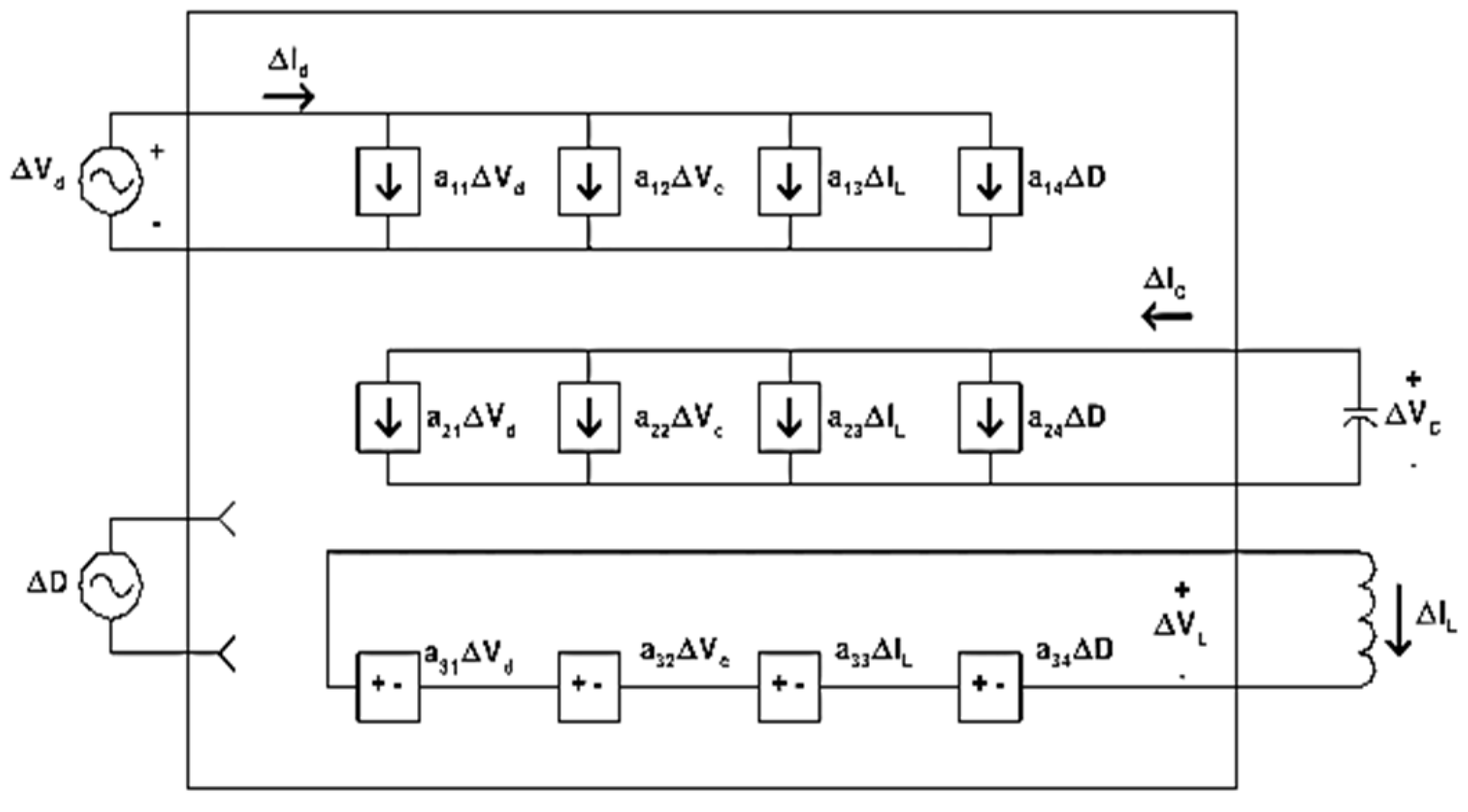
Figure 2.
Averaged small-signal CCM model. A presentation of a circuit that will be used to derive a voltage transfer function.
Figure 2.
Averaged small-signal CCM model. A presentation of a circuit that will be used to derive a voltage transfer function.
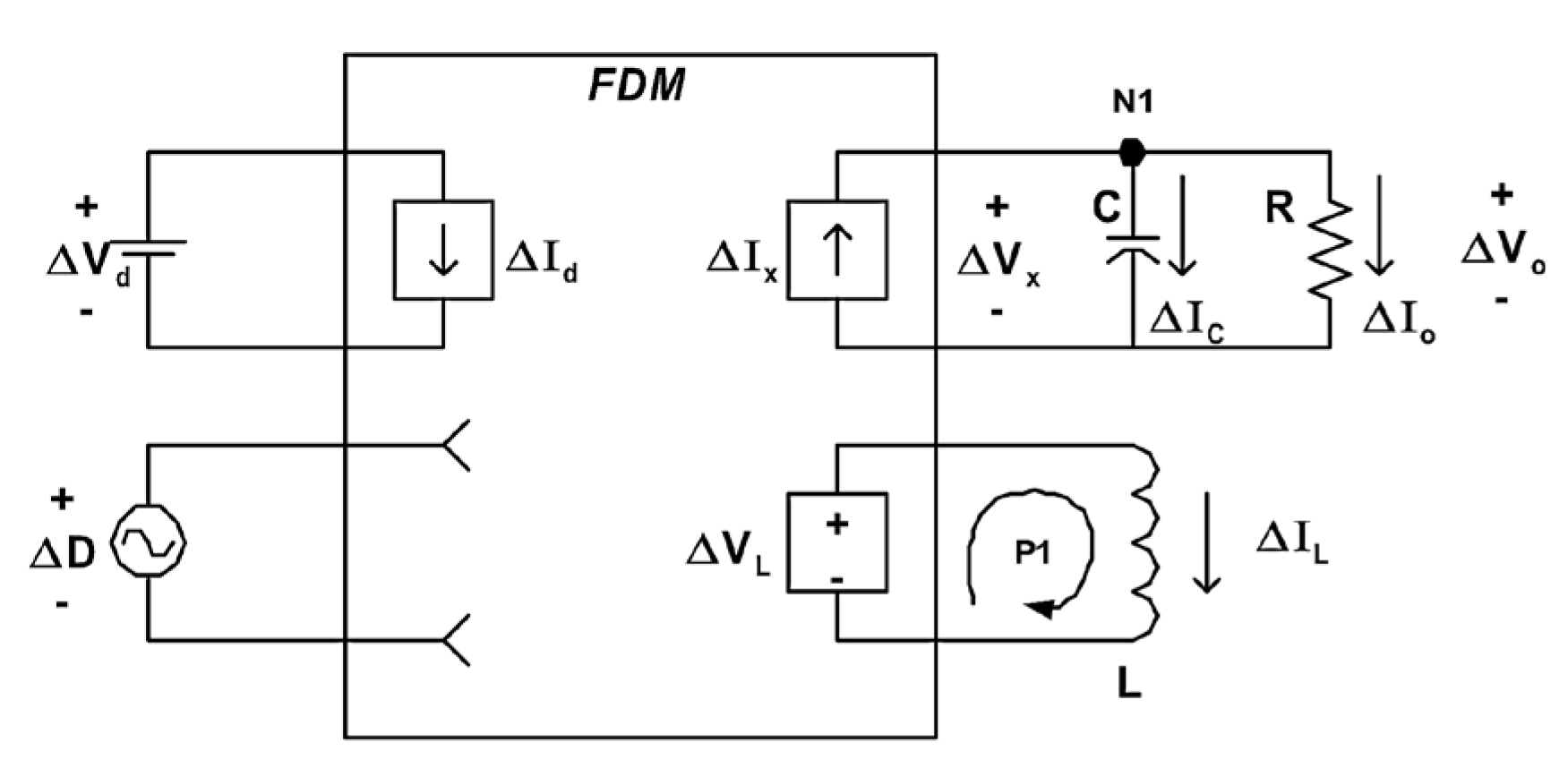
Figure 3.
Classical Buck converter topology. The usual and well-known Buck converter topology for a voltage reduction of a DC-DC converter.
Figure 3.
Classical Buck converter topology. The usual and well-known Buck converter topology for a voltage reduction of a DC-DC converter.
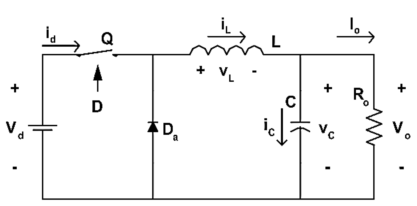
Figure 13.
The transfer function in [dB] is dependent on frequency. A resonant frequency appeared at ƒ=1098.17 Hz, and the transfer function of F(ω)=7.56 dB, as was calculated by the design example.
Figure 13.
The transfer function in [dB] is dependent on frequency. A resonant frequency appeared at ƒ=1098.17 Hz, and the transfer function of F(ω)=7.56 dB, as was calculated by the design example.
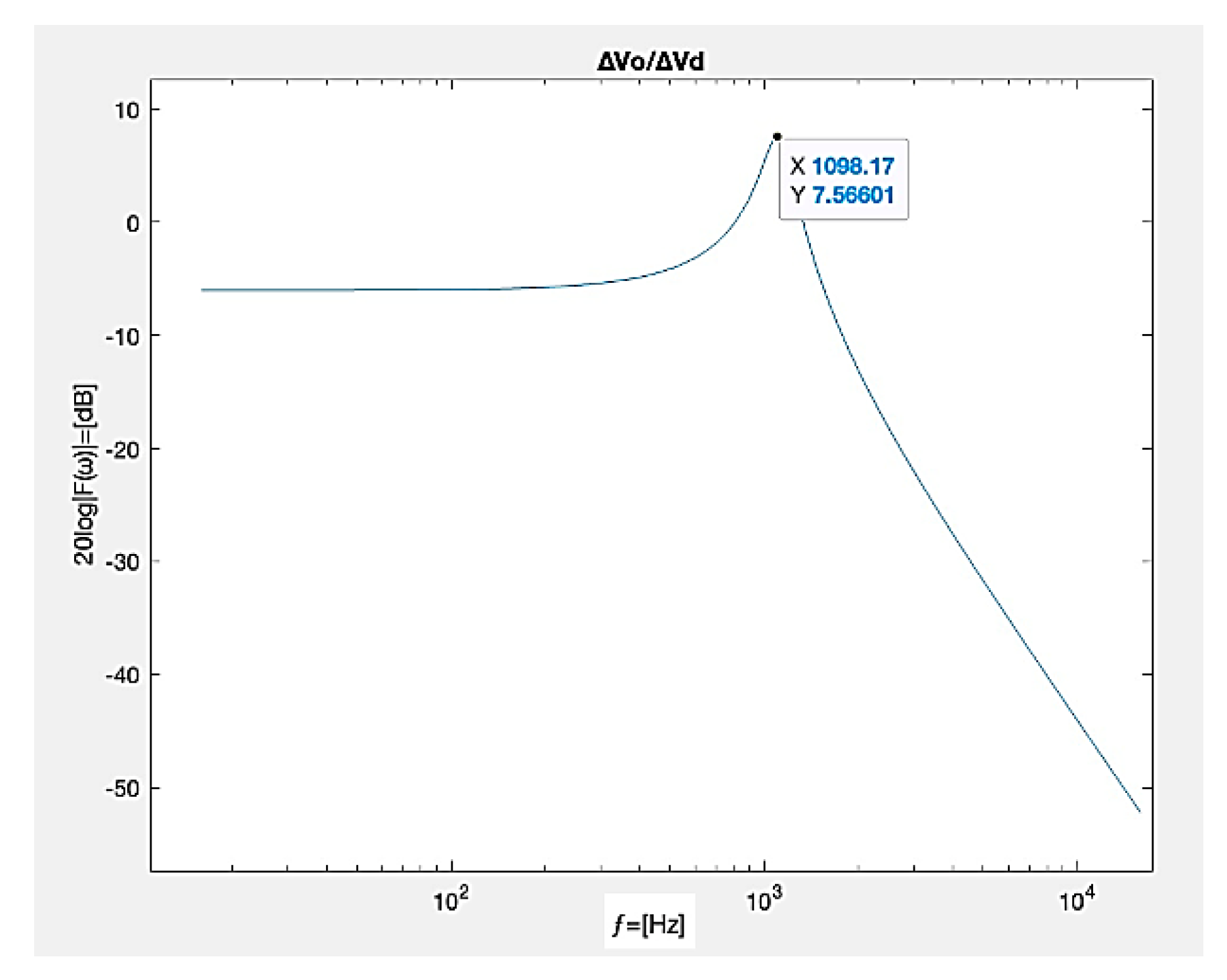
Figure 14.
Basic Buck small-signal model. A model was selected to sharply present the separated voltages DC and AC and designed as a MATLAB model.
Figure 14.
Basic Buck small-signal model. A model was selected to sharply present the separated voltages DC and AC and designed as a MATLAB model.
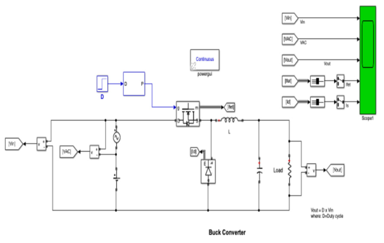
Figure 15.
Input voltage signal of the Buck converter. The FTT presentation yields the DC input voltage of 28V and an AC ripple of 0.5V, as was designed.
Figure 15.
Input voltage signal of the Buck converter. The FTT presentation yields the DC input voltage of 28V and an AC ripple of 0.5V, as was designed.
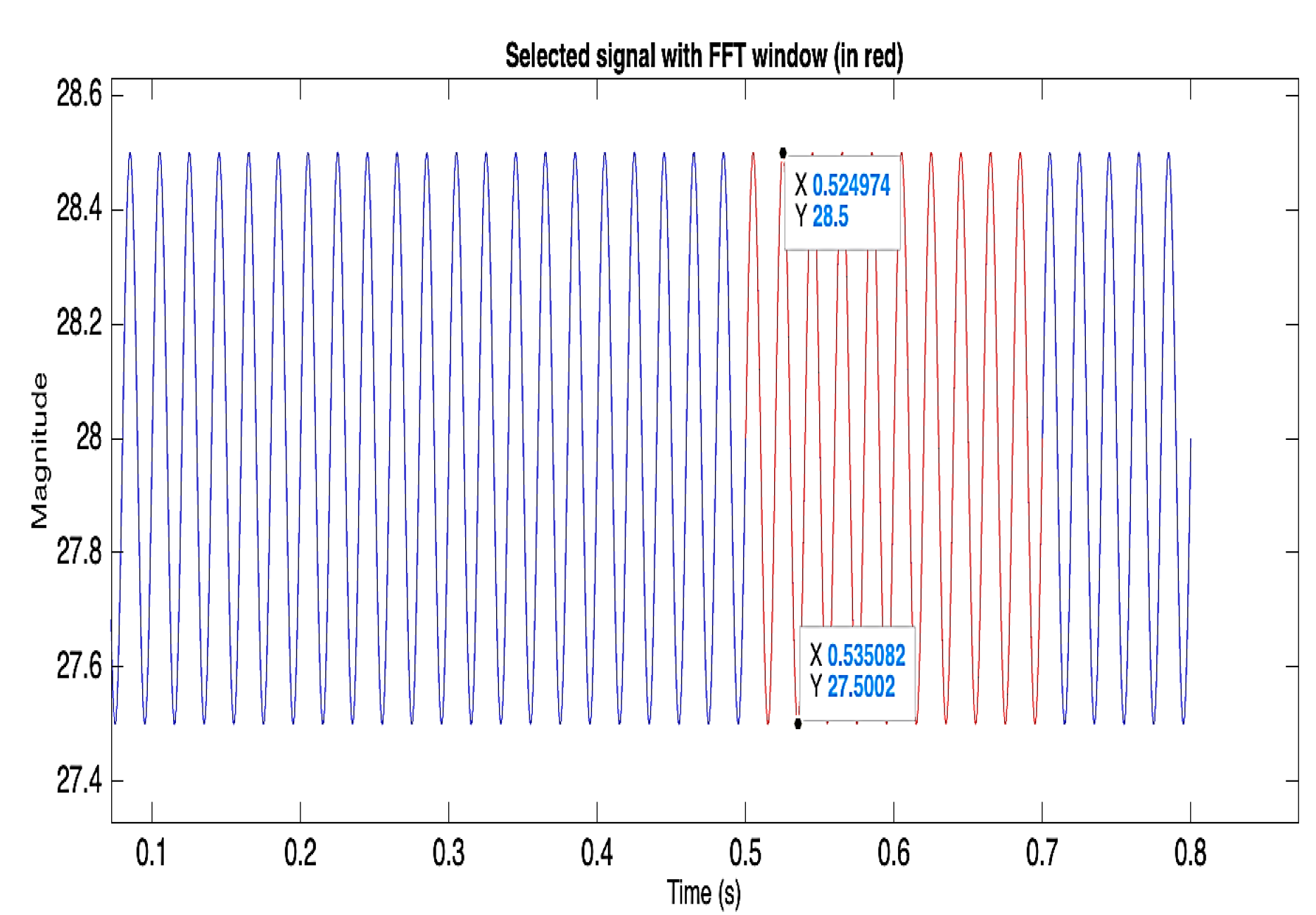
Figure 16.
Output voltage signal of the Buck converter. The FFT picture of an output voltage with 14V DC and 0.25V AC.
Figure 16.
Output voltage signal of the Buck converter. The FFT picture of an output voltage with 14V DC and 0.25V AC.
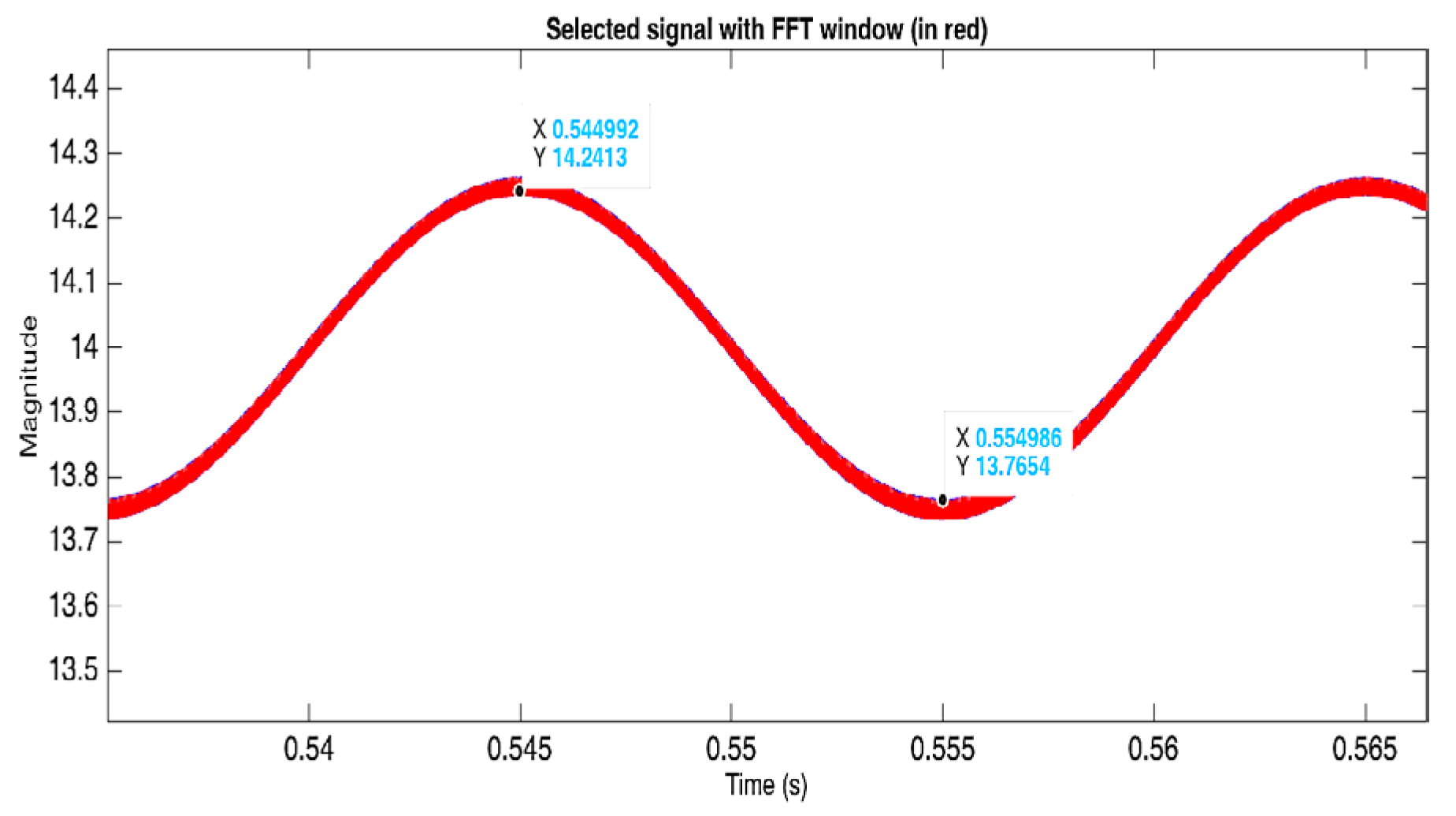
Figure 17.
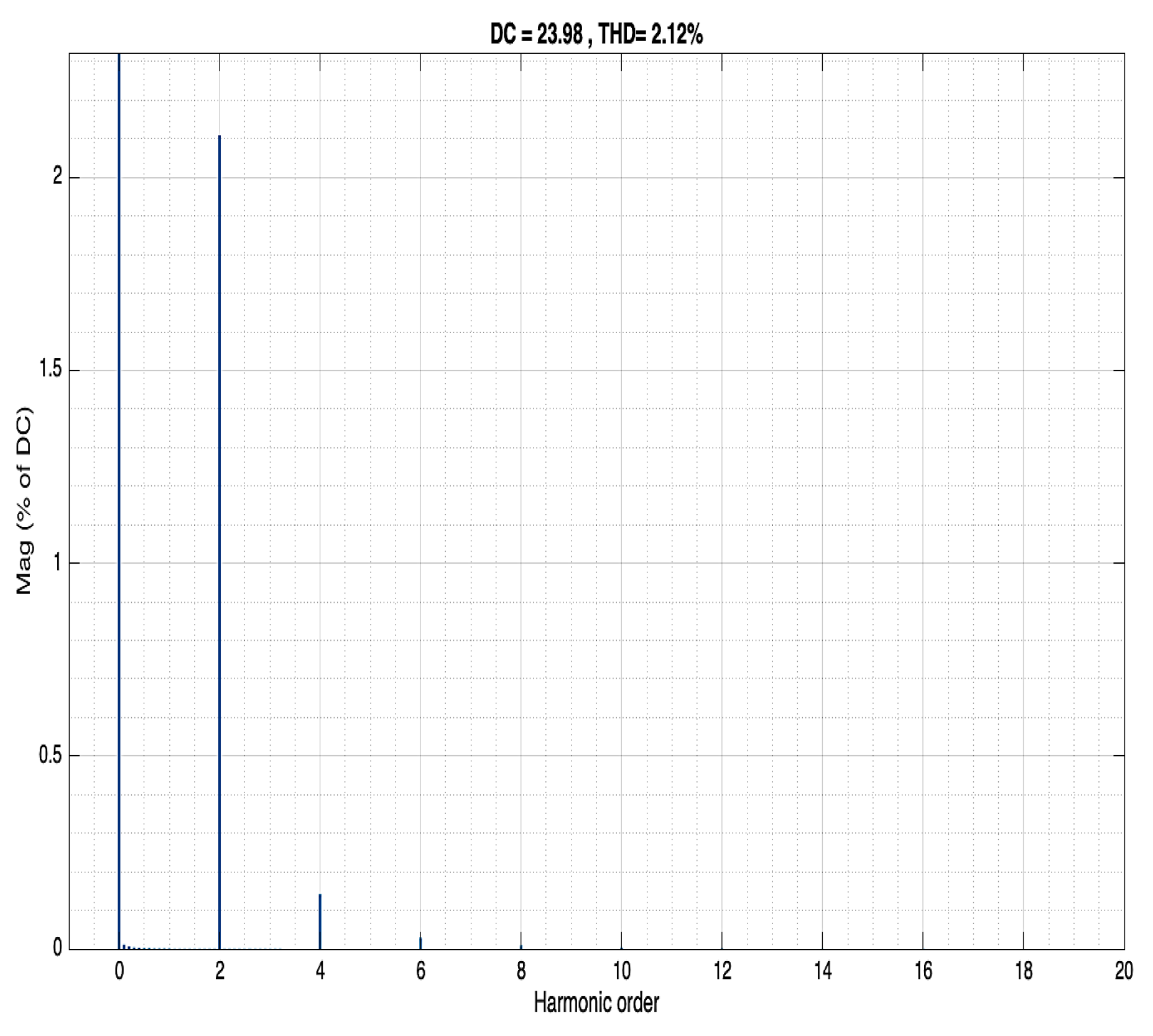
Input voltage as a function of harmonic order Buck converter. A second harmonic's input voltage of 28V and 1.9% THD (at 100 Hz) is an almost perfect AC input.
Figure 17.
Input voltage as a function of harmonic order Buck converter. A second harmonic's input voltage of 28V and 1.9% THD (at 100 Hz) is an almost perfect AC input.
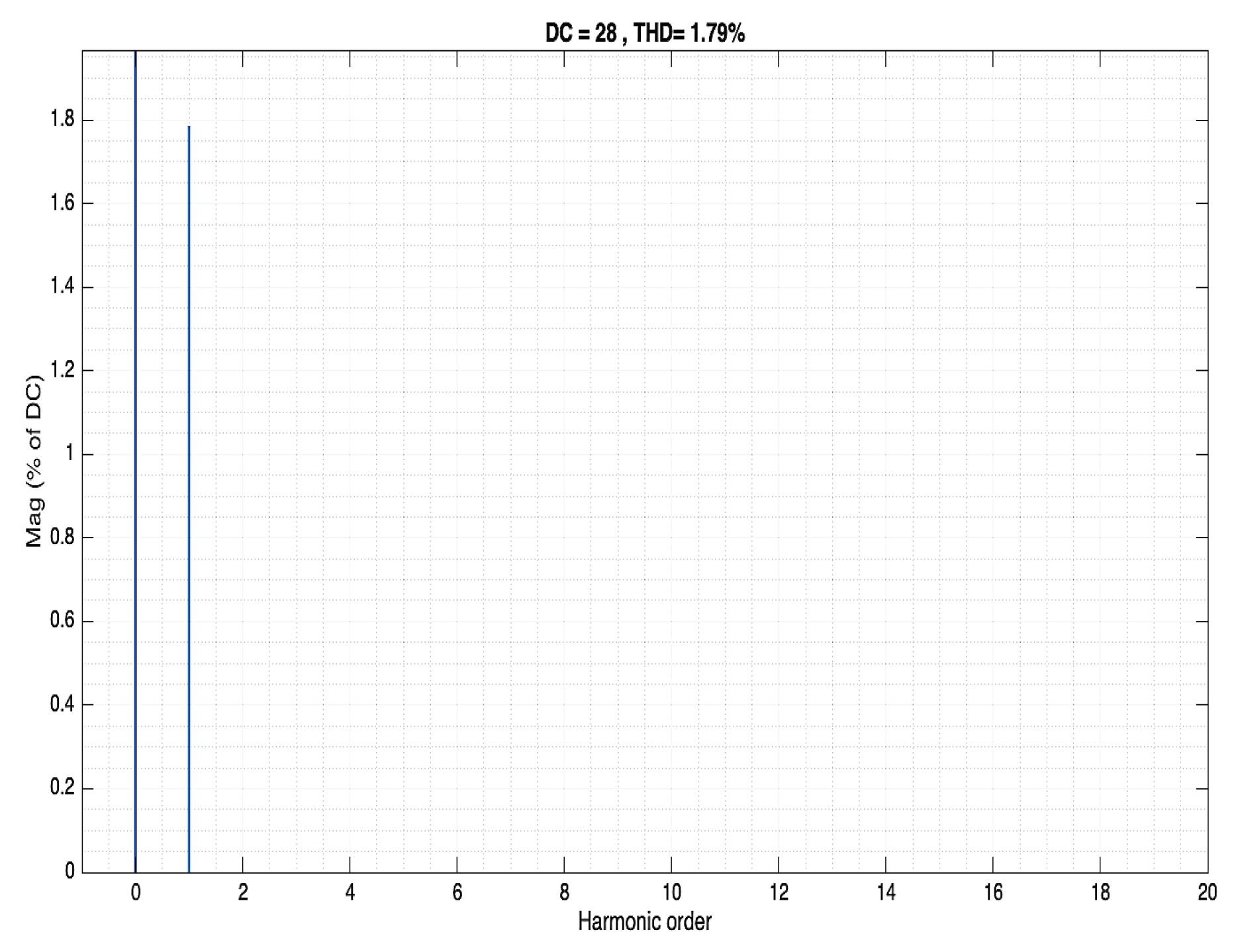
Figure 18.
Output voltage as a function of harmonic order Buck converter. The output voltage second harmonic was transferred unchanged, with the value of 1.9%.
Figure 18.
Output voltage as a function of harmonic order Buck converter. The output voltage second harmonic was transferred unchanged, with the value of 1.9%.
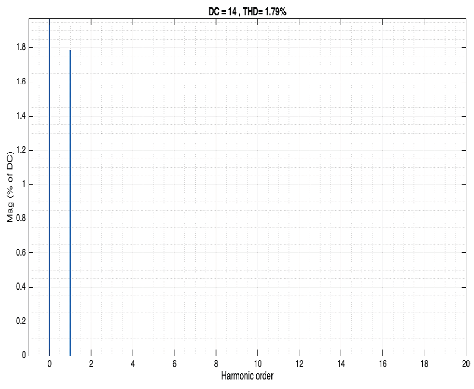
Figure 19.
Transfer function Plot as a dependence of frequency for L=20mH and.
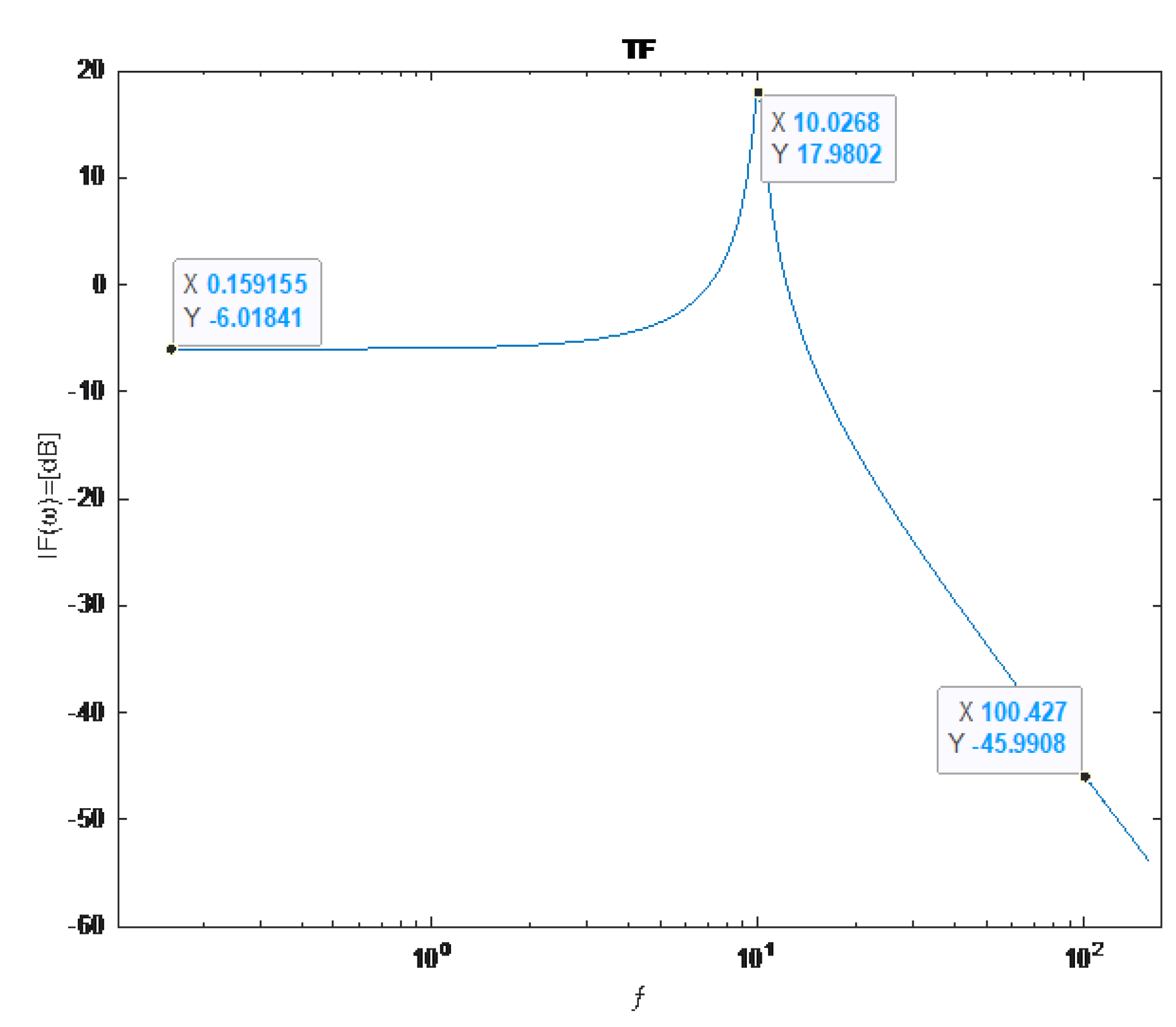
Figure 21.
Buck small-signal model. Compared to the previous design, a more realistic circuit with a full bridge rectifier.
Figure 21.
Buck small-signal model. Compared to the previous design, a more realistic circuit with a full bridge rectifier.
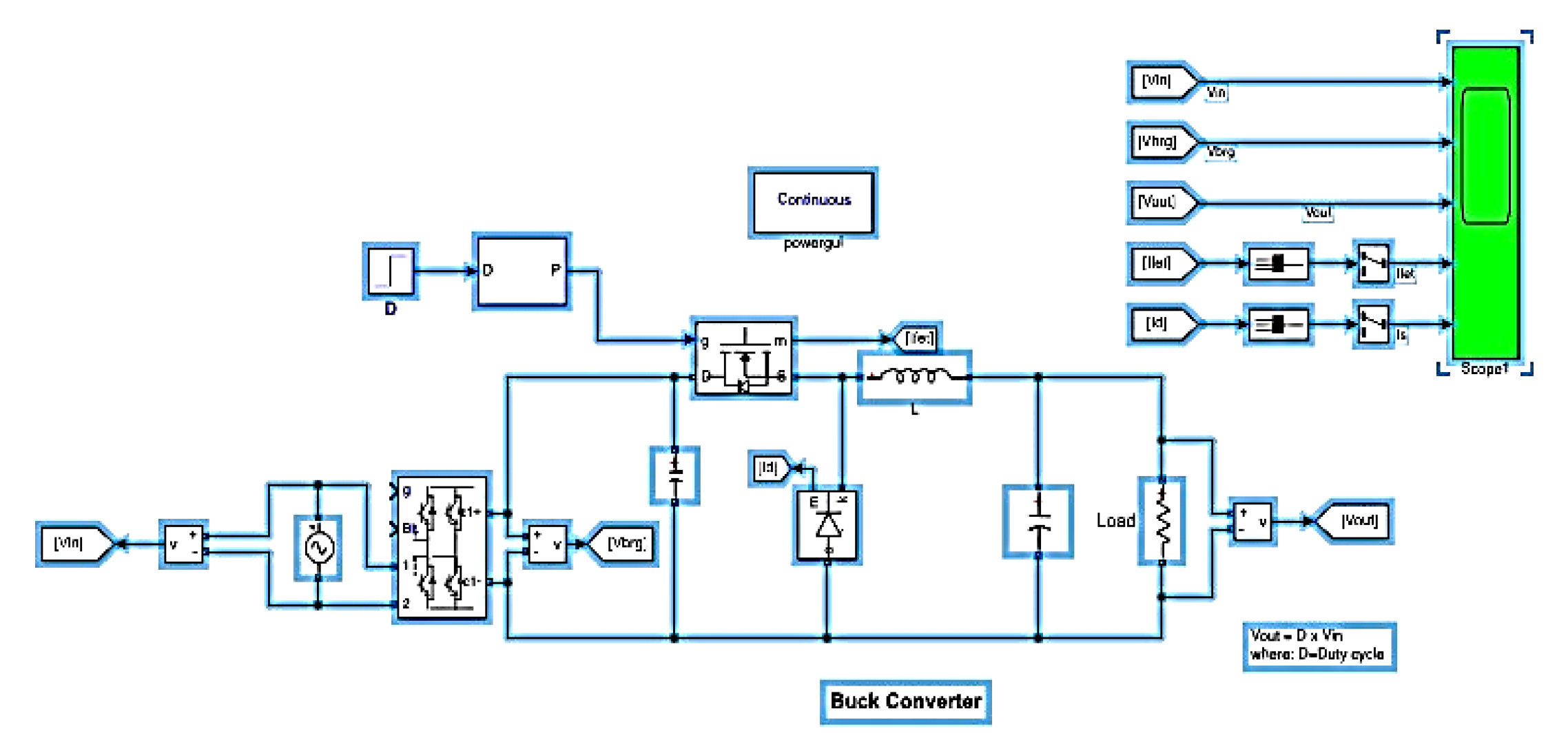
Figure 22.
Input voltage signal. FFT input voltage signal with and with attenuation of
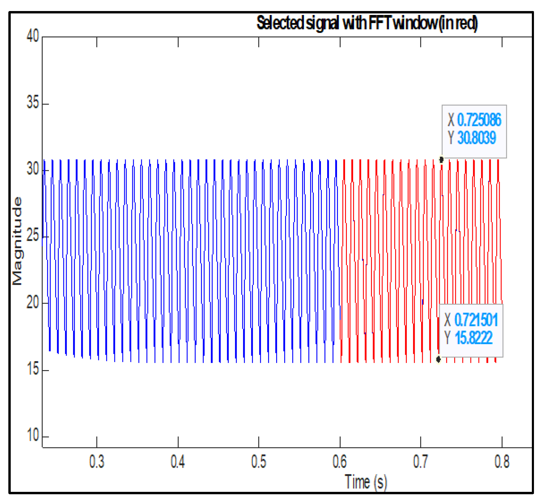
Figure 23.
Output voltage signal. FFT output voltage signal with and with attenuation of
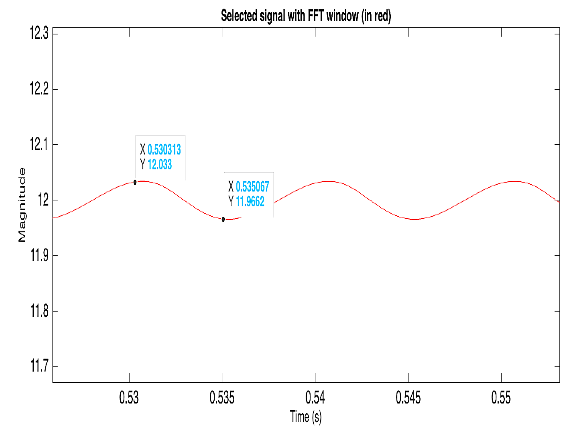
Figure 24.
Input voltage as a function of harmonic order with and C1=12.64mF.
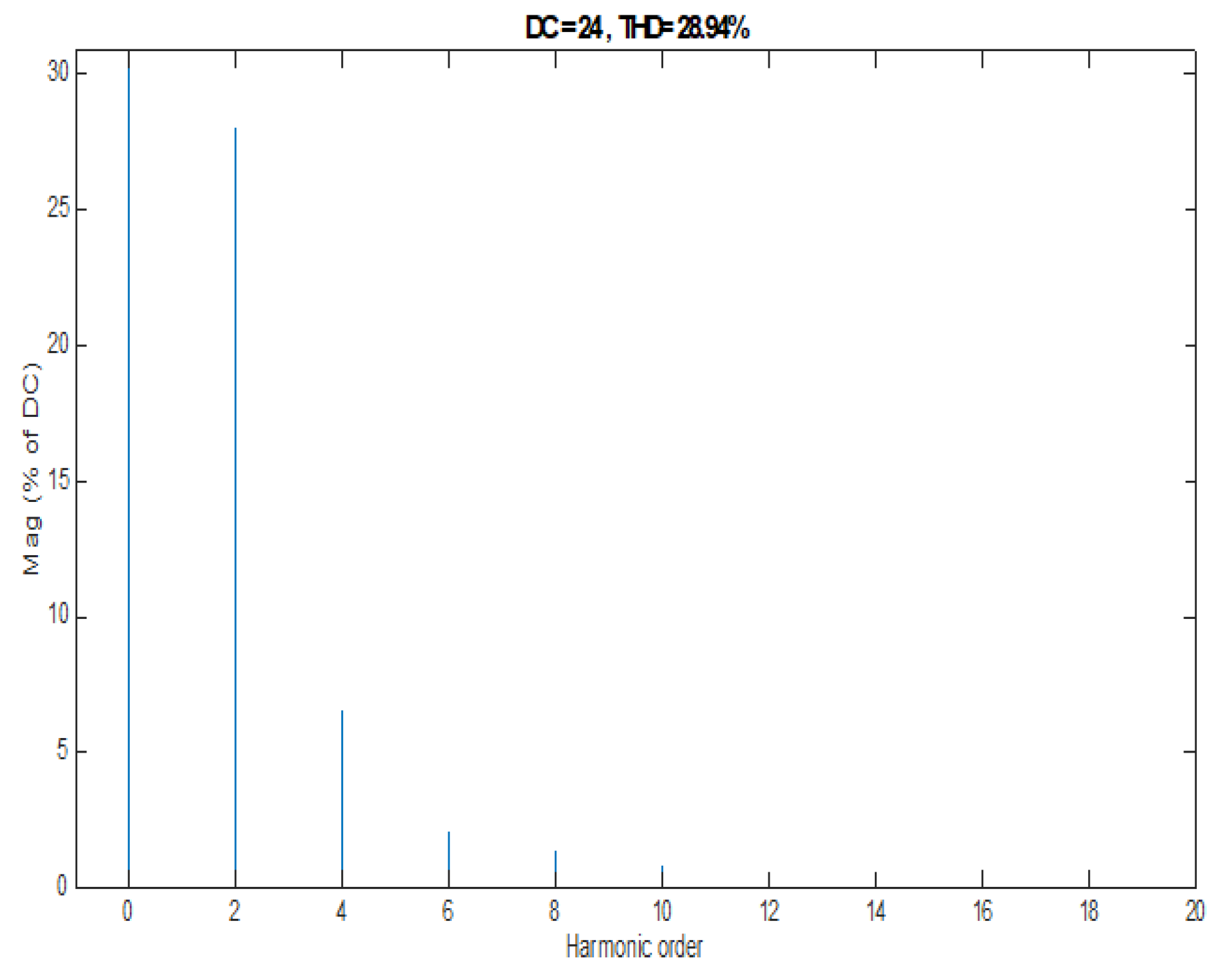
Figure 25.
Output voltage as a function of harmonic order with and C1=12.64mF and attenuation of
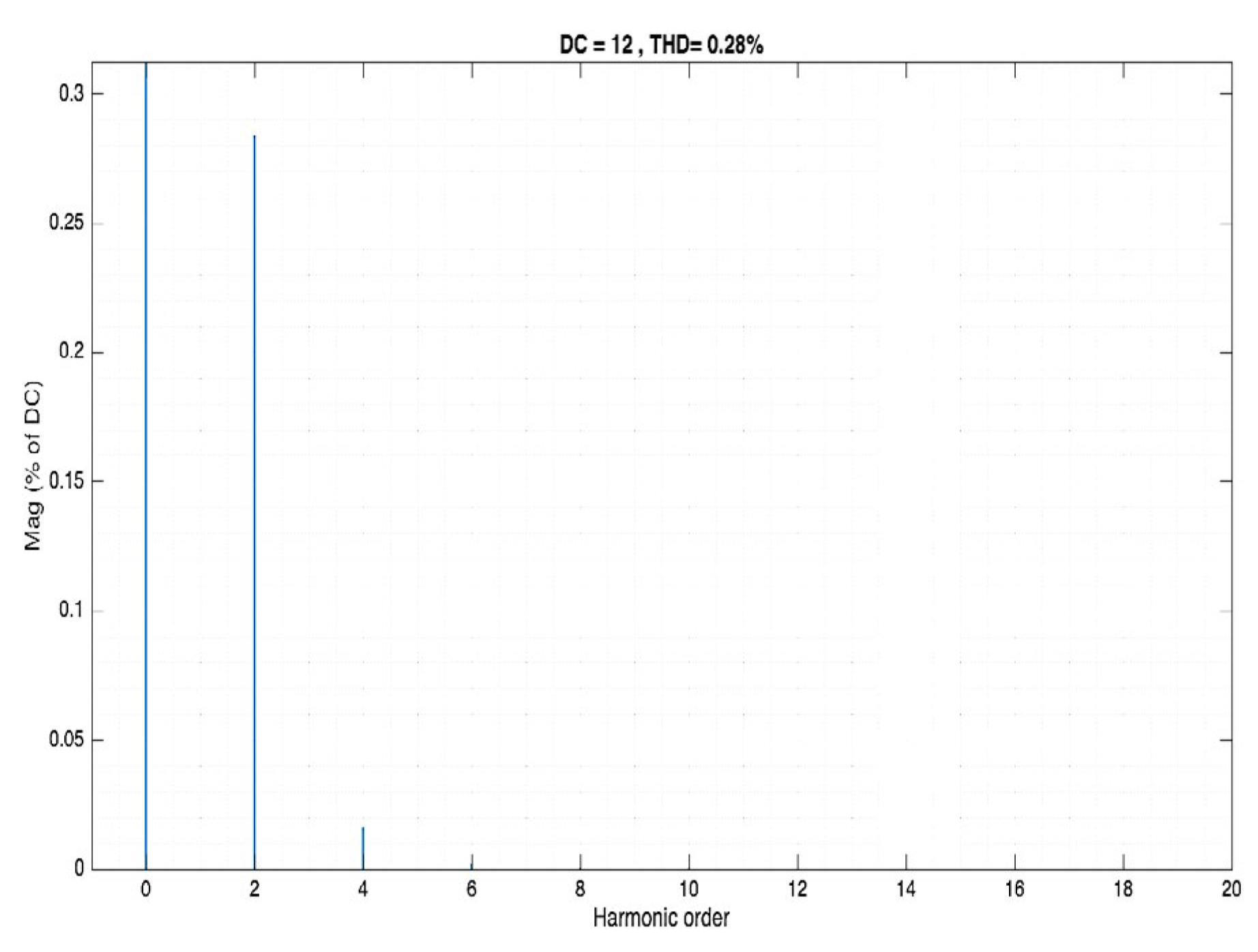
Figure 26.
Input voltage as a function of harmonic order with and C2=25μF.
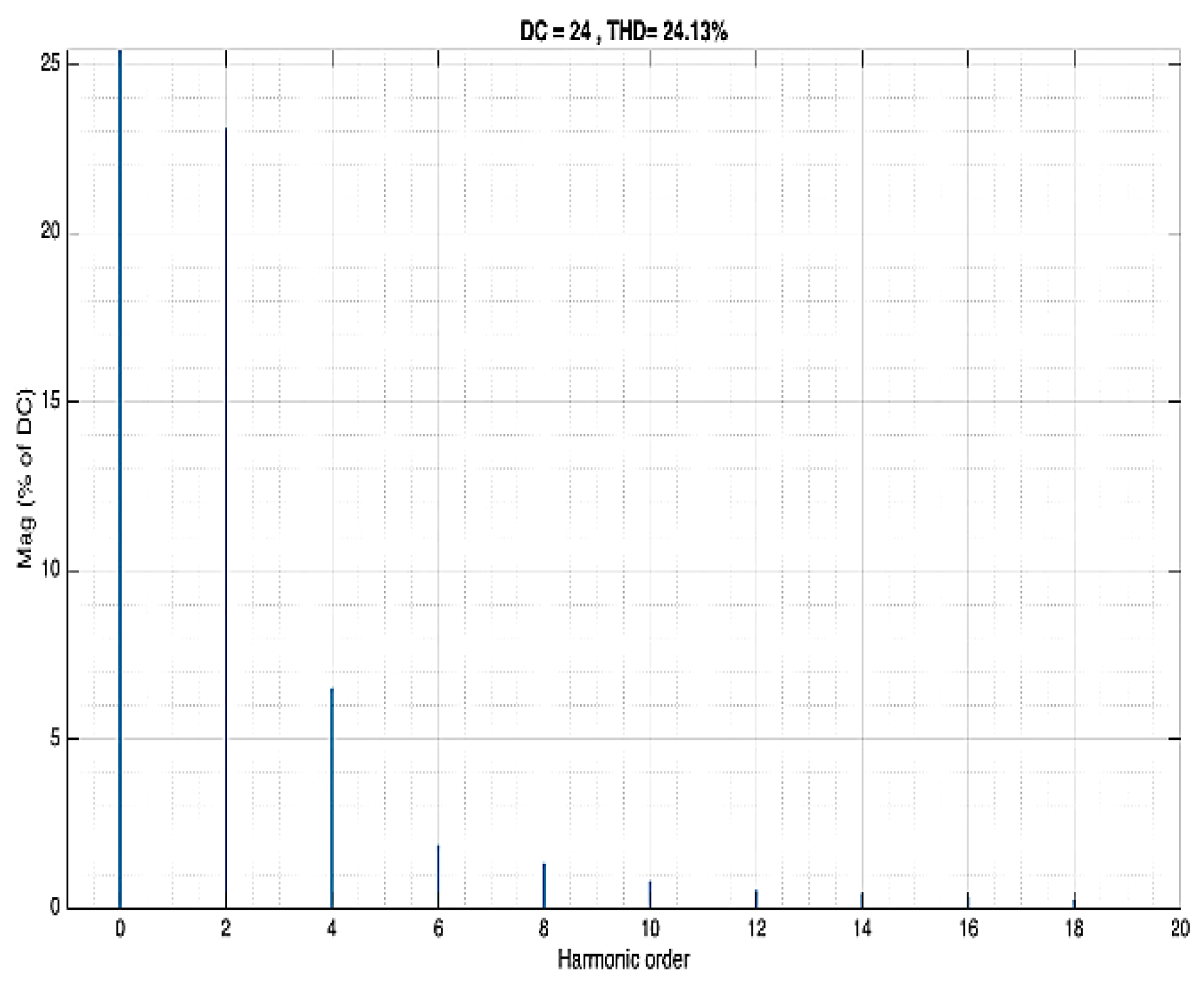
Figure 27.
Output voltage as a function of harmonic order with and C2=25μF and attenuation of
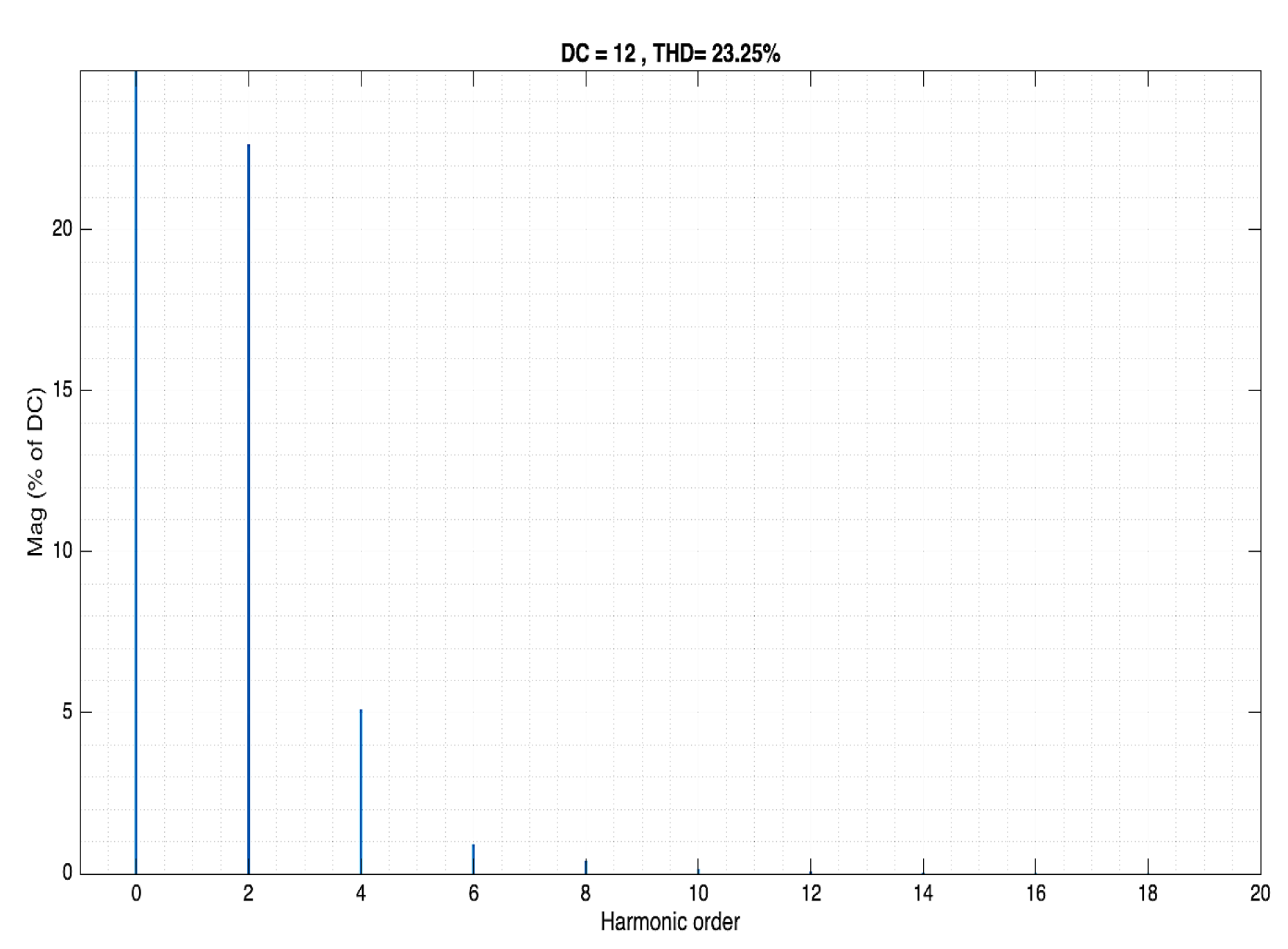
Figure 28.
Transfer function for the Boost converter with components L=20mH and C1=3mF, and attenuation of
Figure 28.
Transfer function for the Boost converter with components L=20mH and C1=3mF, and attenuation of
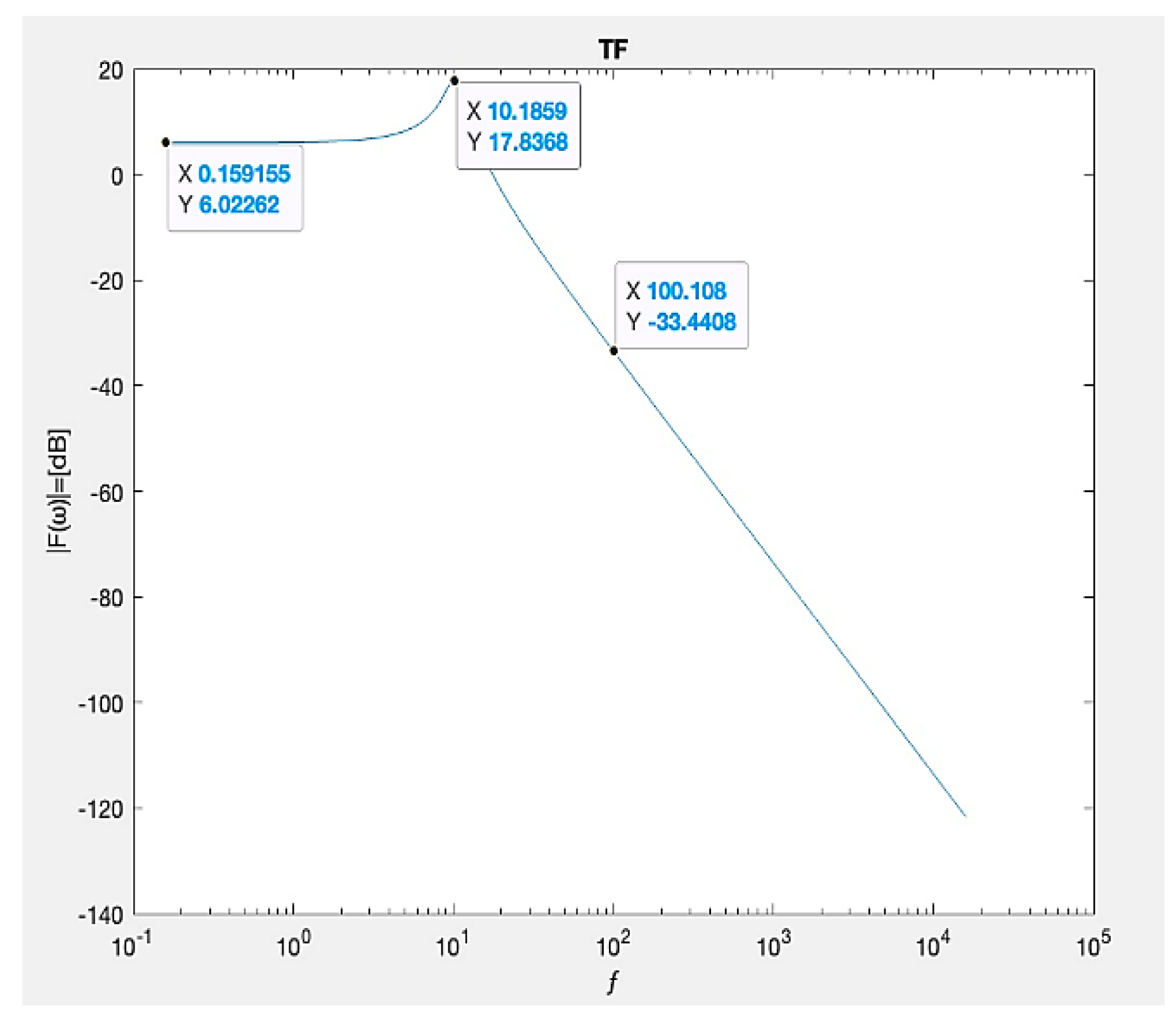
Figure 29.
Transfer function for Boost converter with components L=20mH and C2=103.37μF, and attenuation of.
Figure 29.
Transfer function for Boost converter with components L=20mH and C2=103.37μF, and attenuation of.
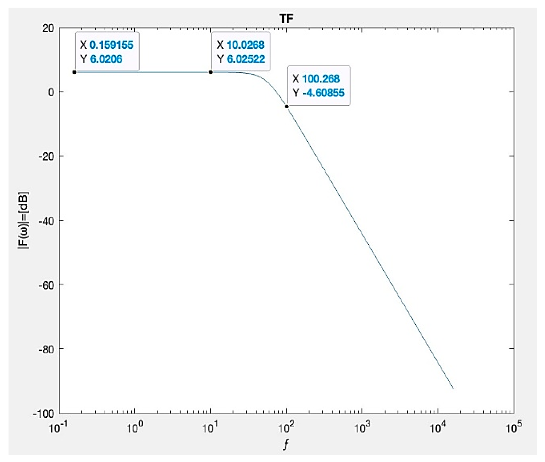
Figure 30.
Input voltage as a function of harmonic order with and C1=3mF.
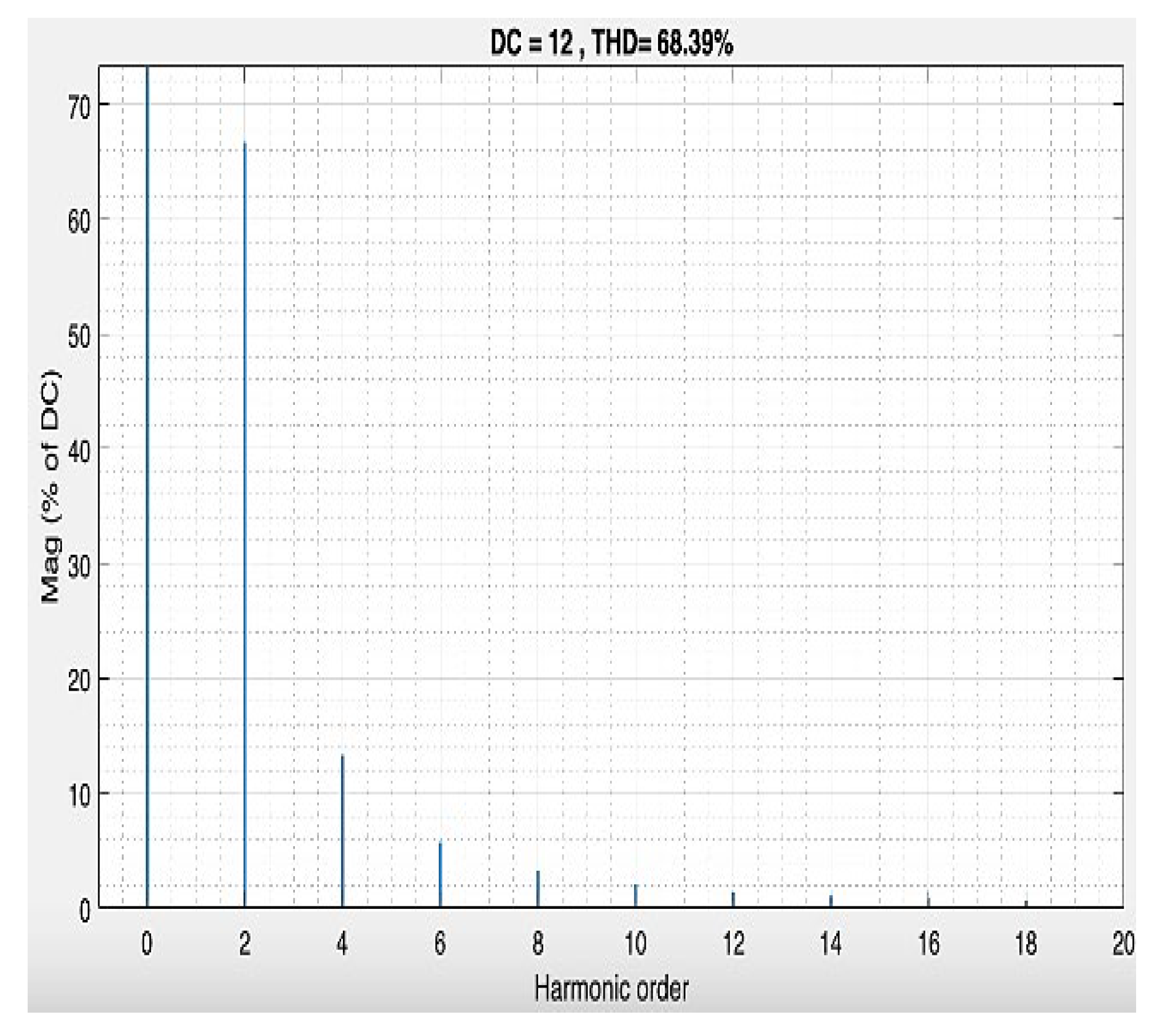
Figure 31.
Output voltage as a function of harmonic order with and C1=3mF and attenuation of
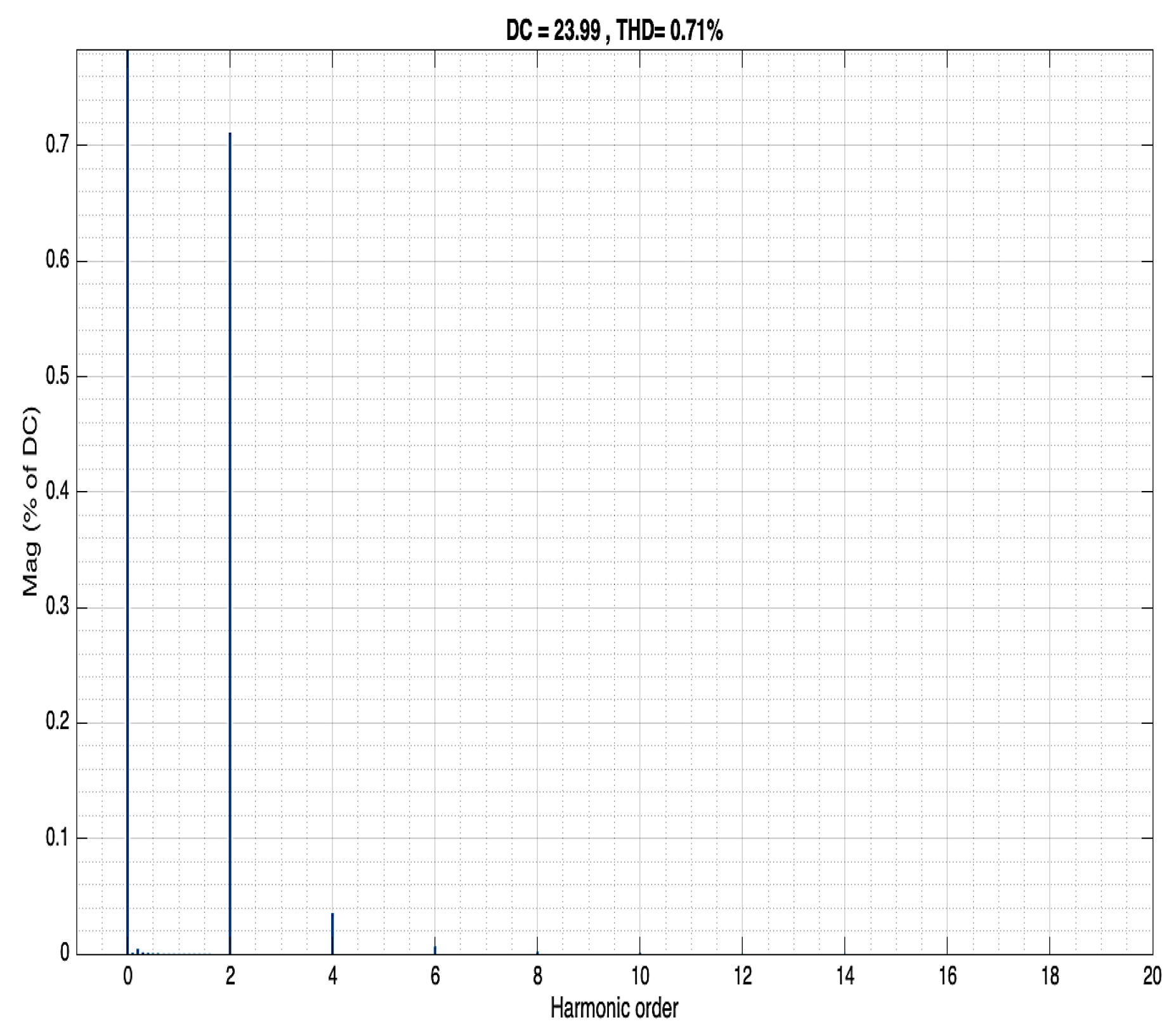
Figure 32.
Output voltage as a function of harmonic order with and C2=103.37μF and attenuation of
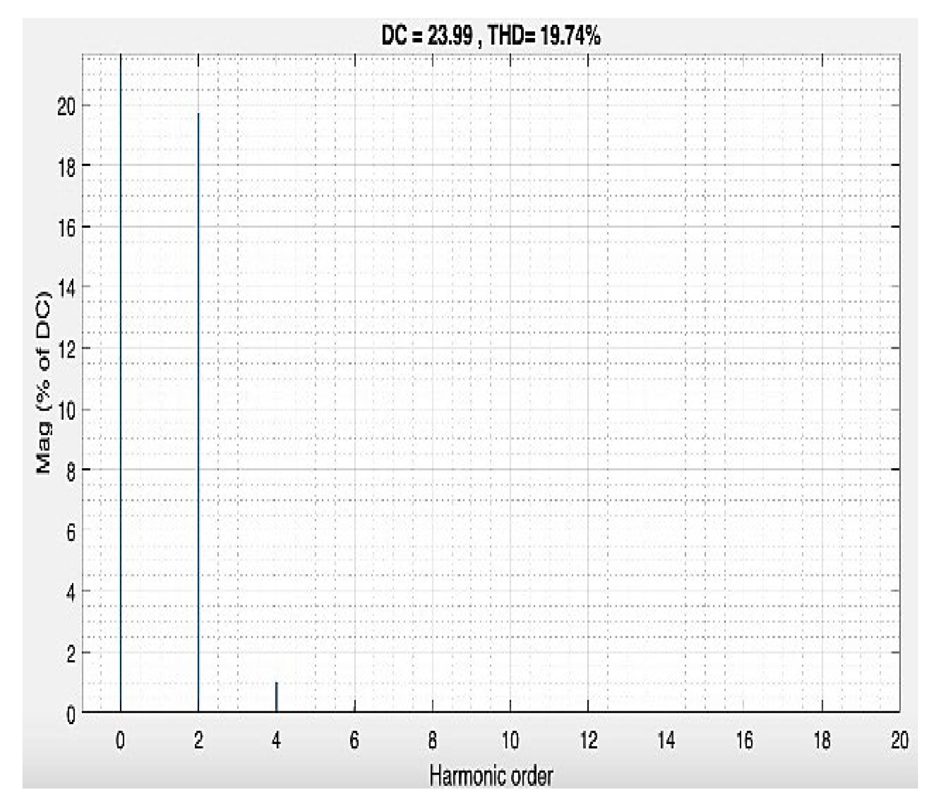
Figure 33.
Buck-Boost converter with components L=20mH and C1=8mF and attenuation of
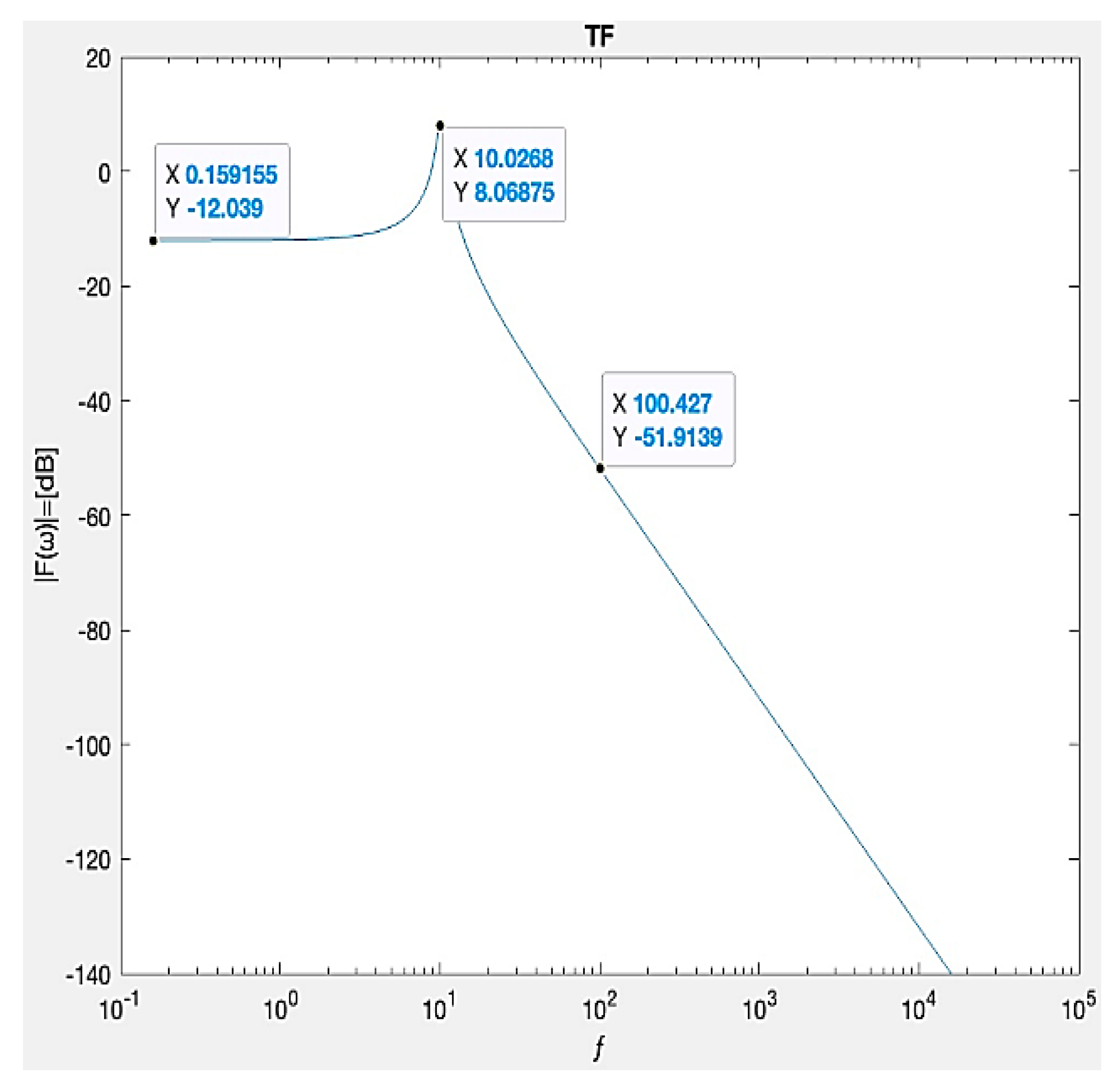
Figure 34.
Transfer function for Buck-Boost converter with components L=20mH and C2=39.25μF, and attenuation of .
Figure 34.
Transfer function for Buck-Boost converter with components L=20mH and C2=39.25μF, and attenuation of .
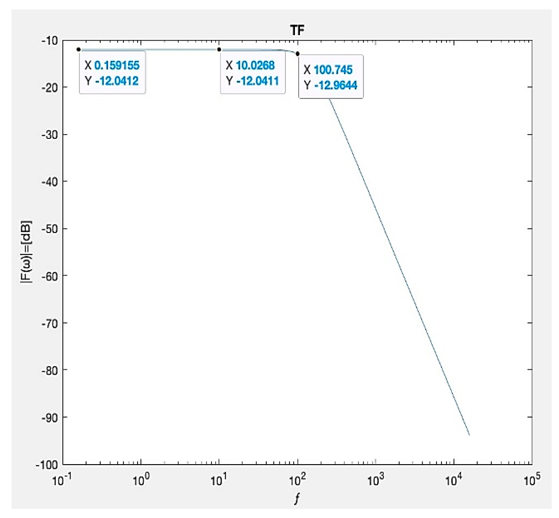
Figure 35.
Input voltage as a function of harmonic order with L=20mH.
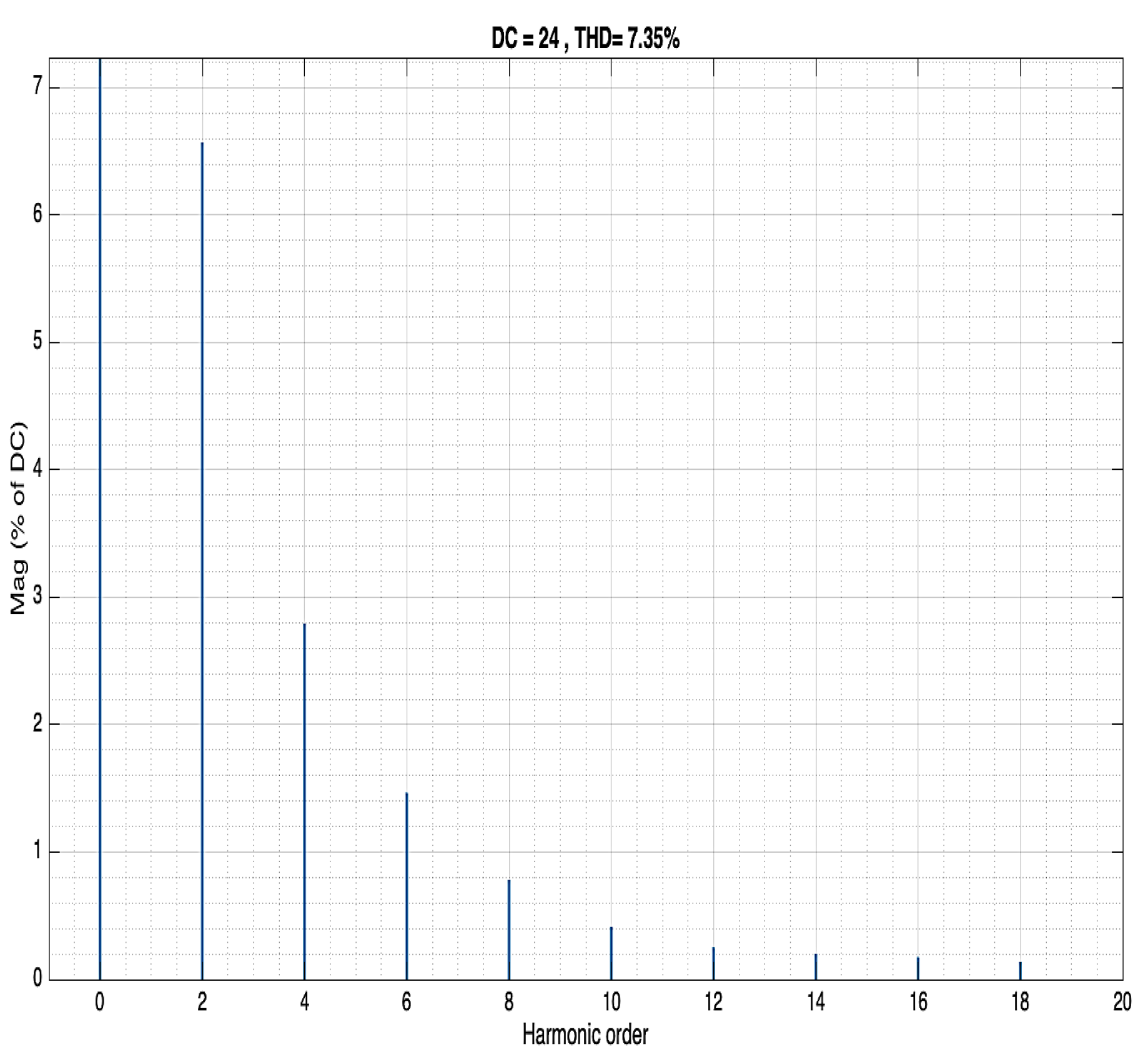
Figure 36.
Output voltage as a function of harmonic order with L=20mH and C1=8mF, and attenuation of
Figure 36.
Output voltage as a function of harmonic order with L=20mH and C1=8mF, and attenuation of
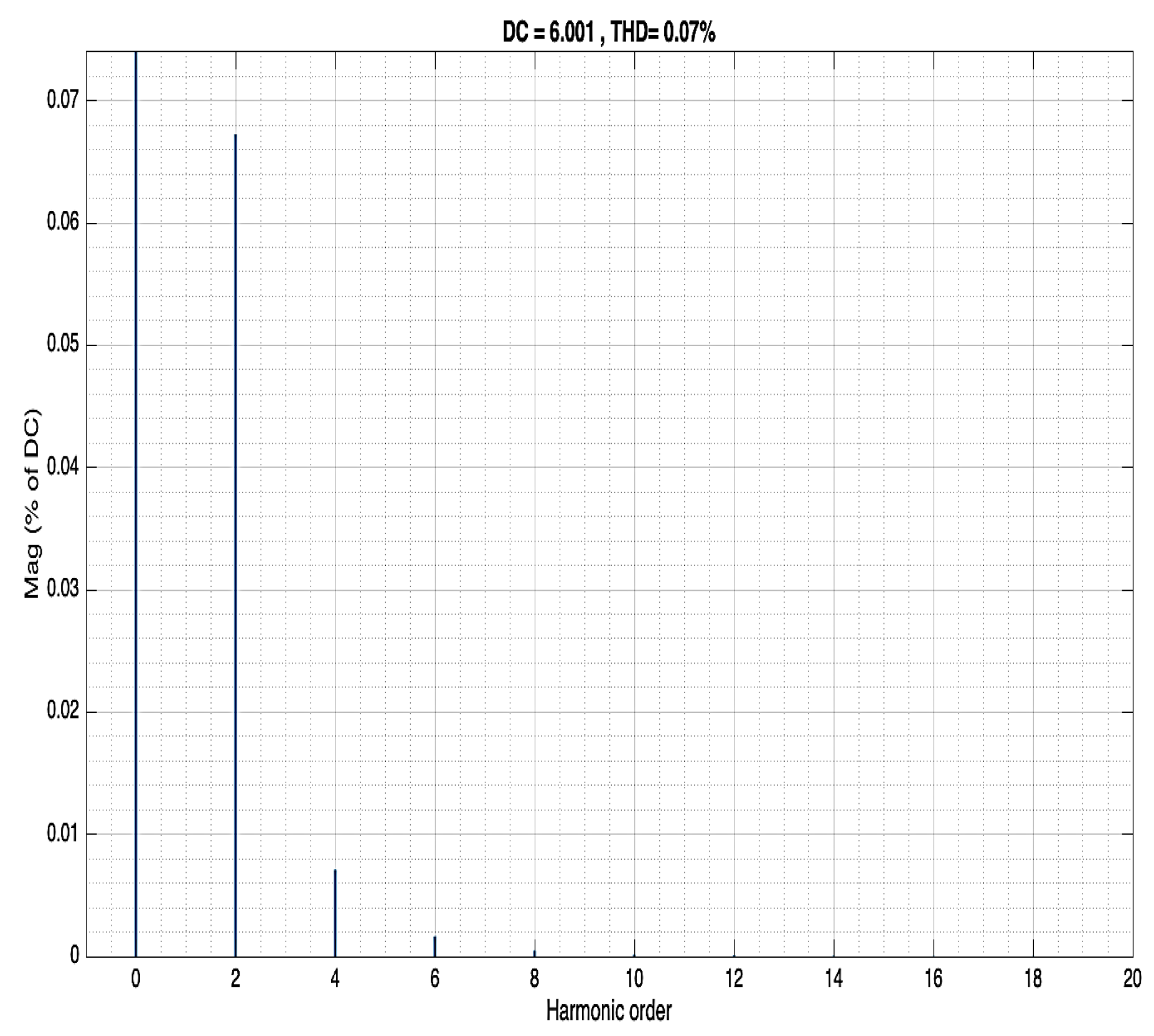
Figure 37.
Output voltage as a function of harmonic order with L=20mH and C2=39.25μF and attenuation of
Figure 37.
Output voltage as a function of harmonic order with L=20mH and C2=39.25μF and attenuation of
Disclaimer/Publisher’s Note: The statements, opinions and data contained in all publications are solely those of the individual author(s) and contributor(s) and not of MDPI and/or the editor(s). MDPI and/or the editor(s) disclaim responsibility for any injury to people or property resulting from any ideas, methods, instructions or products referred to in the content. |
© 2025 by the authors. Licensee MDPI, Basel, Switzerland. This article is an open access article distributed under the terms and conditions of the Creative Commons Attribution (CC BY) license (https://creativecommons.org/licenses/by/4.0/).
Copyright: This open access article is published under a Creative Commons CC BY 4.0 license, which permit the free download, distribution, and reuse, provided that the author and preprint are cited in any reuse.


