

Submitted:
13 November 2025
Posted:
14 November 2025
You are already at the latest version
Abstract
The study given considers a technique for computing the qT-diagram of a multi-flow heat exchanger with an arbitrary number of flows. The specified parameters of the computation are the temperature, pressure, mass rate of all hot and cold flows at the heat exchanger inlet port, and the value of the lowest allowed temperature difference between the flows. The last parameter establishes the heat exchanger's overall thermodynamic efficiency. The algorithm for calculating the qT-diagram includes the calculation of the maximum heat content of the flows, the maximum amount of heat that can be transferred in the heat exchanger, and all possible distributions of this heat between the flows. The outlet temperatures of the flows are computed for each heat distribution, and the results are sorted and ranked according to the chosen objective function. The sorted operating modes of the heat exchanger are checked from the point of view of the qT-diagram's operability in accordance with a given criterion. Comparisons with the results of calculations of similar heat exchangers in the HYSYS AspenONE verified the algorithm's accuracy and physical consistency.
Keywords:
multi-flow heat exchanger
; T-Q diagram
; thermodynamic modeling
; pinch analysis
; algorithm
; process simulation
; cryogenic processes
; second law of thermodynamics
; entropy generation minimization
; heat exchanger network
1. Introduction
Thermal analysis and design of heat exchangers remain among the key problems of engineering thermophysics, particularly in cryogenic and energy systems. The most common engineering tools for such analysis are based on T–Q or T–H diagrams, which relate the temperature of the interacting flows to the amount of transferred heat. These diagrams form the basis of both the classical heat exchanger network (HEN) synthesis methods and modern software packages such as Aspen HYSYS, Aspen Exchanger Design & Rating, HTRI Xchanger Suite, or ANSYS Fluent.
The first formalized methods for analyzing heat exchanger networks trace back to the pioneering work of Hohmann (1971) [1], which laid the groundwork for the seminal works of Linnhoff and Flower (1978) [2]. The latter introduced the pinch analysis technique and the concept of composite curves for two-flow systems, providing an intuitive visualization of thermal interactions and became the foundation for energy-optimal design of exchanger networks. However, the classical pinch methodology is fundamentally limited to two-flow exchangers or equivalent pairwise interactions, where the heat balance can be expressed unambiguously.
In multi-flow heat exchangers (MFHEXs), which are common in cryogenic separation systems, regenerative exchangers, and recuperators with phase transitions, these assumptions fail. Commercial simulation packages such as Aspen HYSYS or HTRI typically treat the problem empirically: users specify temperature differences between the inlet and outlet of each stream, and the program verifies whether the resulting configuration is “operable.” In this process, however, no explicit verification of the second law of thermodynamics is performed at every internal section of the exchanger. As a result, the generated T–Q diagrams may formally appear feasible while actually allowing intersections of the flow temperature curves - a physically impossible scenario.
Other approaches, often found in the literature, are based on local heat transfer equations and the numerical integration of differential equations along the exchanger length (e.g., Ghannadzadeh et al., 2020 [3]; Wang & Xu, 2019 [4]). Although these methods can reproduce detailed profiles of temperature and enthalpy, they require prior knowledge of the exchanger geometry, wall properties, and heat transfer coefficients - parameters that are often unknown in the early thermodynamic analysis stage. Consequently, such approaches are not universal and cannot directly determine whether a feasible heat exchange process exists for a given set of inlet flow conditions.
Entropy-based and exergy-based optimization methods (e.g., Bejan, 1997 [5]) address thermodynamic irreversibility explicitly, yet they are also primarily formulated for two-flow systems or rely on approximating multi-stream exchange as a sequence of binary interactions. This again limits their generality and applicability to real MFHEX configurations.
These limitations motivate the development of a universal thermodynamic algorithm capable of constructing T–Q diagrams for arbitrary multi-flow exchangers without invoking heat transfer equations. The algorithm should:
rely solely on the inlet parameters of all flows (temperature, pressure, mass rate, and composition);
include the minimum allowable temperature difference between any flows as a thermodynamic constraint;
avoid using any geometrical or construction data of the exchanger;
ensure strict compliance with the second law of thermodynamics under all flow combinations.
This method offers a powerful tool for process engineers, enabling them to rapidly screen feasible operating modes and identify thermodynamically optimal configurations for MFHEXs during the conceptual design phase. This can lead to significant reductions in both capital and operational costs by ensuring energy-efficient and physically realizable heat exchanger designs from the outset.
The present study introduces such a method. It is based on the direct thermodynamic analysis of the overall energy balance of a multi-flow heat exchanger, introducing the concepts of active and passive flow bundles. The method involves enumerating all admissible distributions of heat contents between flows, followed by ranking and selection according to thermodynamic objective functions - either entropy-based or temperature-based. The obtained T–Q diagrams, when compared with calculations performed in Aspen HYSYS 12.1, show that the proposed algorithm provides high consistency and physical adequacy without requiring any prior assumptions about heat transfer mechanisms or exchanger geometry.
2. Well Defined Case of a Double-Flow Heat Exchanger
The thermodynamic computation of flow temperatures at the outlets of a 2-flow counterflow heat exchanger (HEX) is a routine procedure for designing different types of refrigeration and thermal engineering equipment. The reasonable accuracy and simplicity of that approach challenge more precise but far more complicated computations based on a set of differential equations relating to hydraulics and heat transfer.
The calculation’s “Thermodynamism” lies in the fact that, for given input flow temperatures , , the outlet temperatures , are entirely determined by the actual amount of heat transferred in the heat exchanger. This can be thought of as a general application of the first law of thermodynamics to the HEX as a whole, without accounting for the specifics of the heat transfer process and the associated design parameters of the HEX.
In the case of ideal heat exchange without losses, the limit amount of heat transferred from hot to cold flow corresponds to the lower of the limit heat content of flows and . The term “heat content” refers to the difference in the total enthalpies of the flow at a HEX’s inlet and outlet ports. The flows limit heat contents and are calculated on the assumption of the equality of the corresponding inlet and outlet temperatures:
here and hereafter, mathematical notations like or imply the use of the corresponding equation of state1.
In the actual real-world scenario case, when irreversible heat exchange losses are to be taken into account, the quantity of heat actually transferred between the TH flows can be defined as a certain fraction of :
where is the coefficient of heat transfer efficiency and its value is set subjectively ( – ideal heat transfer).
It is clear how to calculate the enthalpies and temperatures of the flows at the outlet cross-sections given a known value for :
The heat exchange efficiency coefficient , which was previously provided, is often not employed in engineering calculations to account for losses in the heat exchange process between flows. Instead, the value of the minimum allowable temperature difference at the end of the heat exchanger, , is used. This indicates that the flow’s temperature difference at the heat exchanger’s ends can only be more than or equal to . Using this method, the value of the outlet temperature of one of the streams may be clearly determined based on the ratio of its limit heat contents:
Determine and the temperature of the second flow at the heat exchanger’s outlet using the outlet temperature of one of the flows ( or ) (see eq. (3)).
Both strategies are equally effective and depend only on the individual. Similar to , the particular value of is selected based on personal preference. The maximum value is constrained by the values of the inlet flow temperatures, while its lowest value is set within (3 .. 6), K. However, when doing numerical computations of the flow temperatures along a HX’s length, it may be beneficial to set strict, clear limits on the range of values .
The thermal load (see eq. (3)) uniquely determines the values, in any of these calculation alternatives, and it is a priori assumed (without verification) that the condition:
holds for each cross section of the HEX.
The last assumption is valid for a limited number of cases when the dependences and for working substance flows remain close to linear in the corresponding temperature ranges: , . This means that the above-mentioned approach should only be used in situations where there are no phase transitions occurring during the heat exchange process and flow temperature variations of no more than a few tens of degrees.
If the dependences or are nonlinear in the temperature ranges that are being studied, then computations should be done not only for the flow temperatures , at the heat exchanger’s outlet but also along the entire length of the heat exchanger, based on the quantity of heat transferred:
then determining if the requirement has been met.
The Tq-diagram of HEX (see Figure 1) is the graphical depiction of dependencies (6).
Algorithm to Compute the 2-Flow Heat Exchanger’s Tq-Diagram
The Tq-diagram of the two-flow HEX must be calculated after figuring out and (eq. (1), (2)) and their corresponding flow temperatures at the HEX’s outlets and (eq. (3)).
Then the entire HEX is divided along the length into n sections. To ensure that the thermodynamic properties of the flows and evolve in a nearly linear fashion over each segment, a particular value of n is to be selected.
Usually, n is chosen such that the temperature changes by 5 to 10 degrees along a section , and then the total number of sections n: . The sections are numbered starting from the inlet port of the cold flow: . The flows’ temperatures and enthalpies are then computed for all HEX’s sections.
If the temperature difference between the hot and cold flows in each internal cross-section of the HEX is greater than a predetermined value , then the Tq-diagram is deemed to be operational (the appropriate values of the HEX’s ends temperature differences are established earlier; see eq. (3), (4)):
Figure 1 presents three alternatives for the Tq-diagram of two-flow HEX calculated with input data from Table 1. Based on the HEX’s heat balance (eq. (1)) and idealized conditions of transferring the maximum possible amount of heat in the HEX 73.2, kW; (eq. (2)) the diagram in Figure 1A was created. In this instance, the condition of a zero-temperature difference between the flows at one of the HEX’s ends—here, the cold end—is automatically met. It is believed that the observed intersection of the temperature curves in Figure 1A violates the second rule of thermodynamics, indicating that such a process is physically impossible to carry out under any heat transfer scenario. In actuality, it means that under the set initial data, it is impossible to transfer a given quantity of heat from a hot to a cold flow. In this scenario, either the lowest allowable HEX’s end temperature difference or the coefficient of heat transfer efficiency should be decreased in order to lower (see eq. (2), (4)).
In Figure 1B, the Tq-diagram is likewise computed for the idealized heat transfer process in the HEX, but under the condition that (see eq. (9)), which is the minimal allowable value of the temperature difference between the flows in any internal cross-sections. In this instance, 66.9 kW of heat is transferred in the HEX. This is the maximum quantity of heat that can be transferred in the HEX under these initial data without going against the second law of thermodynamics. The operational diagram of the HEX, computed for the constraint = 5 K, is shown in Figure 1C. The amount of heat transferred in the HEX is = 62.8 kW, or 93% of its maximum value of 66.9 kW.
It is evident that the value of but not should be the basis for the iterative calculation of both the Tq-diagram and the HEX’s efficiency. However, given the constraint , the computation of the value requires an extensive iterative computation of the Tq-diagram in itself (see (9)). Consequently, the value is used as the maximum heat load for calculation of Tq-diagrams employing the concept of the HEX’s thermal efficiency . This very slightly increases the number of iterations; otherwise, it has no effect on the final computation results. Wherein, the value should clearly be used to evaluate the effectiveness of a HEX: .
3. A multi-Flow Heat Exchanger Case Study
The above-discussed two-flow heat exchanger is a special case of a multi-flow heat exchanger (MFHEX), where several hot and cold flows undergo simultaneous heat exchange. The set of all hot flows of a MFHEX will be referred to as a hot bundle for brevity, and the set of all cold flows as a cold bundle. Calculating the Tq-diagram of a two-flow HEX does not contain any particular difficulties since the amount of heat given off by the hot flow at each heat exchange section is equal to the amount of heat absorbed by the cold flow, either taking into account possible losses or without them in the case of ideal heat exchange. In the thermodynamic calculation of a MFHEX, there is no such unambiguous relationship between the amount of heat transferred between flows, since thermodynamics does not operate with such concepts as heat transfer coefficients and heat transfer surface area. The latter significantly complicates the procedure for calculating the Tq-diagram of MFHEXs.
As in the case of a two-flow HEX, the first step is to determine the amount of heat transferred in the MFHEX from all hot flows to all cold flows.
We will assume that each of the hot flows is in the process of heat exchange with each of the cold flows and can only emit heat. To avoid a situation where any of the hot flows may turn out to be colder than any of the cold flows, we accept the assumption that there is a limiting temperature for hot flows at the MFHEX’s outlet ports. None of the hot flows can have a temperature lower than , and this temperature will correspond to the temperature of the “hottest” of the cold flows at the MFHEX’s inlet ports:
Following the same logic, the limiting temperature for cold flows at the outlet of the MFHEX will correspond to the temperature of the “coldest” of the hot flows at the inlet to the heat exchanger:
The assumption of limiting temperatures , implies the presence of limiting heat contents in flows , . The values of , and of a MFHEX’s hot and cold flows are entirely determined by the limiting temperature values and , given the input parameters:
here and hereafter, mathematical notations like or imply the use of the equation of state corresponding to a working fluid of the specific flow.
Any MFHEX flow’s real heat content must be larger than zero (because we believe that every flow inevitably exchanges heat with other flows) and less than or equal to the value of its limiting heat content:
The limiting heat content of the hot and cold bundles of a MFHEX (recall that a MFHEX’s bundle is a set of either all the hot or all the cold flows) is the sum of the limiting heat content of the flows included in the bundle:
The smaller of the limiting heat contents (16) of the bundles is the maximum quantity of heat that may be transferred between bundles (i.e., all hot flows with all cold flows):
Let us designate as an “active bundle” MFHEX’s bundle of flows with a greater maximum heat content and a “passive bundle” (of flows) with a lower maximum heat content. A bundle’s “activity” or “passivity” is only based on its maximum heat content ratio, not on whether it is hot or cold.
The quantity of heat that is actually transferred between the flows of a MFHEX’s bundles may be calculated as a certain fraction of , much as in the case of a two-flow HEX, when irreversible losses in the heat exchange process are taken into consideration:
(see eq. (2))
The total heat transferred in a MFHEX is removed from all hot flows:
and distributes (disperses, scatters, divides) among all cold flows:
Passive Bundle
First, let’s consider the perfect heat transfer with no losses . In this case, the amount of heat released (or received) by each of the passive (with a lower maximum heat content) bundle’s flows will obviously equal the maximum heat content of the flow (eq. (12) or (13)). Here, the outlet temperature of the flow is equal to its corresponding limiting temperature or . The distribution of the total heat amount transferred between the bundle flows is then known:
| Passive bundle | Heat transfer in a MFHEX without losses: ε = 1 | |
| Hot | (20) | |
| Cold | (21) |
Now, we assume that the relationship (eq. (20) or (21)) that was calculated for the case of ideal heat exchange still holds true when there are irreversible losses in the heat exchanger: and . Next, using the values of or the amount of heat released (or received ) by a distinct flow of the bundle and the temperature of the flows at the outlet (or ), will be computed:
| Passive bundle | Heat transfer in a MFHEX with losses: ε < 1 | |
| Hot |
|
(22) |
| Cold |
|
(23) |
Active Bundle
By definition, the limiting heat content of the active bundle (or ) exceeds the amount of heat actually transferred in a MFHEX. Consequently, the heat content of each of the flows of the active bundle cannot simultaneously be equal to its limiting values, as in the case of a passive bundle. Specific values of (or their ratio) are not defined and depend on the conditions of heat exchange between flows, the thermophysical properties of the flow substance, phase state, mass flow rate, etc. Only the ranges of changes in the heat content of the flows are known with certainty: , subject to the condition .
Since thermodynamic calculations of heat transfer do not use either the heat transfer equations or the actual concepts of heat transfer coefficients and heat transfer surfaces, it is impossible to directly calculate either the specific values of (or ) in eq. (18), (19), or the temperature of the active bundle flows at the outlet ports of a MFHEX. As a brute-force method in this case, a set of values of allowable heat contents from the range can be set for each flow of the active bundle. From these sets of , every potential combination of active bundle flows’ heat content (, , …, ) that corresponds to the condition can be obtained. Since the heat content and temperature of the passive bundle flows are already known by this moment (see eqs. (22), (23)), it becomes possible to calculate the Tq-diagrams for a MFHEX for all the sets (, , …, ) obtained. The results of the calculation are to be examined (sorted) in accordance with the given criteria. Such criteria might include one of the following: the minimum difference between the actual and limiting values of the flows’ temperature at the MFHEX’s outlet ports; the lowest possible irreversibility in the heat exchange processes between the flows (the minimum value of the rate of entropy production in an MFHEX); etc.
An Array of Feasible Heat Contents for an Individual Flow
It is technically more convenient to combine shares of the active bundle flows heat content (with in mind that the active bundle can be either a “hot” or a “cold” one) rather than their actual values :
Let’s set the minimum value of , the same for all flows in the bundle: . The maximum value of may vary from flow to flow, and its specific value is determined by restrictions (14), (15) on the heat content of the flow. The ban on the zero heat content of the flow (in fact, this is a ban on the “non-participation” of the flow in heat exchange) means that depends on the number of flows N in the bundle, since :
Taking into account the second restriction, which states that , is contingent upon each flow specific parameters and is limited to the following value:
The smaller of and is chosen as the actual value, :
Thus, for every flow of the active bundle (refer to eqs. (16), (17)), a vector , can be assigned:
In eq. (28) you can set the value the same for all flows. Then the increment in :
can vary from flow to flow. You can keep the same for all flows, but then the vectors will have different lengths:
Both choices are equal and valid.
A set A is a useful way to express the collection of vectors that are calculated for each active bundle ‘s flow :
The set A consists of vectors that are typically diverse in their length .
A Set of all Feasible Distributions of the MFHEX’s Overall Heat Load Between the Flows
The set A will be used to produce a set of all feasible and physically consistent distributions of the thermal load between the flows of the active bundle: .
Let us construct a vector of length such that every element , corresponds to one of the elements of the vectors of set A that are iterated successively, say for example, . Such a vector fully characterizes one of the various distributions of the thermal load across all flows of the active bundle if the total of all components of this vector equals 1 (see eq. requirement (24)).
In order to obtain a set B of all possible options for distributing the thermal load between the flows, one must first find all possible combinations of elements of the vectors of set A with each other. The well-known combinatorics technique—the Cartesian product of a set with itself—will be used to achieve this:
Consequently, we are left with a set B made up of > vectors, each of length , which is equal to the number of flows in the active bundle. In general, the sum of the elements of an arbitrary vector of the set B may differ from 1. By eliminating from the set B all the vectors for which the condition is false, we may reduce the set B to its subset C:
Set C contains < elements that represent vectors of all possible distributions of the thermal load between the flows of the active bundle (precisely to the magnitude of , see eq. (29)). Fulfillment of the condition means that each vector will correspond to the heat balance condition for the flows of the active bundle (24): .
The transition from the heat content fractions in the set C to the (T, h, s)—parameters of the active bundle flows at the exit from the MFHEX—is as follows:
| Active bundle | Heat transfer in a MFHEX with losses: ε < 1 | |
| Hot |
, see eq. (10) ; |
(34) |
| Cold |
, see eq. (11) ; |
(35) |
The parameters and are directly employed in equations (34), (35) to compute the MFHEX’s Tq-diagrams, and the differences and are used to first sort the set of potential solutions, which will be covered below.
By successively applying the relevant equations (34) (or (35)) to every element in set C, we can derive a set D of potential parameters for the active bundle flows at the MFHEX’s exit:
Each array of output parameters of the active bundle flows in the set (36) taken together with the set of invariable output parameters of the passive bundle flows (refer to eqs. (22) and (23)) specifies some operating mode of a MFHEX. This data is sufficient to calculate the Tq-diagram of the mode.
By going successively from vector to vector in (36): D1, D2, …, DD, Tq-diagrams for every operational mode of MFHEX may be computed. After all the diagrams are analyzed further, only the most suitable diagram will be chosen based on performance evaluation criteria (see Algorithm to compute the 2-flow heat exchanger’s Tq-diagram). This strategy has clear costs. It makes sense to first sort the MFHEX’s operating modes that match the vectors (36), based on the objective functions or reported below. We will calculate Tq-diagrams for a set of sorted vectors up to the first operable diagram.
Objective Functions or to Rank the MFHEX Operational Modes
According to the principles of thermodynamics, an ideal heat transfer process is the one that is reversible and generates either zero or very little entropy. Consequently, operating modes of heat exchangers with a smaller total change in the entropy of flows are thermodynamically more preferable because they mean lower losses during heat exchange. Now let’s put down the objective function related to the MFHEX’s change in flows entropy:
For every element-vector in the set (36), is calculated and then all the elements of are sorted using the rising function :
The minimal difference between the actual temperature values (see eqs. (34) –(36)) of the active bundle flows at the MFHEX’s outlet and their upper limit values (see eqs. (10) and (11)) might serve as an alternate criterion for the heat exchanger’s efficiency:
Since the outlet temperatures of the passive bundle flows (see eqs. (22) and (23)) do not change throughout the computations, the objective function (39) can be applied only to the outlet temperatures of the active bundle flows.
The minimum value of the function implies that the outlet temperatures of the active bundle flows have values as close as possible to their limiting value: , with the minimum possible “scatter” of their values around : .
As in the case of , is computed for every vector element in the set (36) and the elements are then sorted using the increasing function :
It should be emphasized that, in contrast to the situation of minimizing the function , the objective function may be computed simultaneously for all flows of the active bundle, for flows that have been individually chosen, or even for a single flow if necessary.
Algorithm to Compute the Multi-Flow Heat Exchanger’s Tq-Diagram
Just as in the case of 2-flow HEX, the MFHEX is divided into n sections along its length in order to calculate the Tq-diagram:
where is the flows temperature increment (decrement) within one section. The specific value of , let’s say, 10 K is chosen subjectively, based on the consideration that the nature of the change in the flows’ thermodynamic properties within each individual section is about to be linear.
At this point, the outlet parameters of the passive bundle flows have already been calculated and are assumed to be unchanged for all operating modes of the MFHEX (see (22) and (23)). The set of potential outlet parameters of the active bundle flows is also calculated and sorted (see eqs. (38) or (40)) in accordance with the selected objective function. Let us recall that any of the MFHEX’s modes of operation is completely determined by a set of outlet parameters of the active bundle flows (grouped in arrays of the set or ) and a set of invariable outlet parameters of the passive bundle flows.
To find out if a certain MFHEX operating mode has an operable Tq-diagram, you need to figure out the distribution of the flow enthalpies and the corresponding temperatures (where k is the flow cross-section) for the outlet parameters of the flows that go with that mode:
For all pairs of -hot () and -cold () the MFHEX flows, the temperature differences in all sections are determined: . Next, the minimal temperature difference for each pair, and the heat exchanger as a whole, , is chosen:
The MFHEX operating mode and the Tq-diagram that goes with it are said to be operational when the following condition is met:
Here, is the minimum temperature difference that is allowed between MFHEX flows.
If condition (45) is not met, then calculation (42)-(45) is to be repeated for the next operating mode of the MFHEX, the next vector-array Di of set (38) or (40).
If condition (45) is not satisfied for any of the elements of the set (eq. (38)) or (eq. (40)), then this means that, under given initial conditions, the amount of heat (see eqs. (16)-(18)) cannot be transferred from all hot to all cold flows under any heat transfer conditions. In order to get a feasible Tq-diagram, it is necessary to decrease by lowering the heat transfer efficiency coefficient (eq. (2)).
4. Validation of Calculation Results
The presented algorithm for a MFHX Tq-diagram calculation has been translated into computer code for Python v. 3.5. The code exploits a set of numerical computer subroutines developed by the National Institute of Standards and Technology (NIST) 2 to calculate thermodynamic and transport properties for various fluids and mixtures.
We carried out calculations of Tq-diagrams of 2- and 3-flow HEXs for a number of values of the minimum allowable temperature differences between flows. The acquired data was validated by comparing it to the results of calculations of similar heat exchangers in the Aspen HYSYS 12.1 program3.
4.1. 2-Flow HEX
The initial data for cold and hot flows in a 2-flow HEX4 is presented in Table 1. We want to point out that in order to compute the Tq-diagram, one also needs to define the lowest allowable temperature difference between the flows (see eqs. (9) and (45)) and the error δε in determining the HEX’s coefficient of efficiency (see (2)). The following computation results were all acquired with an error of δε = 0.0001.
We consider the Tq-diagram of the heat exchanger to be “operable” if the minimum temperature difference between the flows is greater than or equal to the specified value . The calculation and analysis of “operable” diagrams occurs in the range of the HEX’s efficiency using the golden section method until the condition is met: . If this condition is met, the Tq-diagram for εmax will be “inoperable” (the minimum temperature difference between the flows is less than the specified ), and for εmin it will be “operable”.
The following calculations are presented in Table 2, depending on the specified minimum allowable temperature difference between the flows:
- ∘
- the HEX’s efficiency:
- ∘
- the amount of heat transferred in the HEX;
- ∘
- the temperature differences: at the HEX hot end (
- ∘
- cold end ();
- ∘
- the minimum calculated temperature difference between the flows inside the HEX.
In the course of the computation, the operating modes were sorted and ranked using the objective function (eq. (37). The computation results for the objective functions (eq. (37)) and (eq. (39)) coincide in the case of the 2-flow HEX. Figure 1C and Figure 3 provide a graph of the computed Tq-diagram of the 2-flow HEX in the scenario when = 5 K.
The results of calculating a similar 2-flow HEX in the AspenTech HYSYS AspenONE 12.1 program are presented in Table 3.
To calculate the Tq-diagram of the HEX, AspenTech allows you to set any values of the temperature difference between the flows at either the hot or cold ends of the HEX (see [7]). Apparently, the program does not analyze the limiting heat content of the flows and overlooks the possibility of the objective existence of a minimum temperature difference between the flows at one of the HEX’s ends, under which one can’t go down.
A user manually goes through the possible values of at either the hot or cold end of the HEX until he receives an operable Tq-diagram with the required value of the minimum temperature difference between the flows.
A satisfactory correlation is observed between the values of the HEX’s efficiency and the quantity of heat that is actually transferred in the HEX with a change in given in both calculations (see Table 2 and Table 3). The values of and computed by the reported program and HYSYS showed a relative difference of (1-2), %, and (4.6–6.1), %, respectively.
At the same time, the discrepancies between the corresponding values of the end temperature differences () with changes in are noticeably greater and amounted to: for the hot end (5.4–7.0), %, and for the cold end (25.4–37.6), % (see Figure 2). Reducing the temperature step along the flow by increasing the number of nodes n (eq. (41)) on the flow computational grid did not improve that situation.
Figure 3 compares the Tq-diagrams of the considered 2-flow HEX, calculated in our program and in HYSYS for = 5 K. As can be seen from the temperature curves, the HEX’s cold flow does not change its phase state, and both calculation programs show negligible differences in the distribution and range of temperature changes throughout the length of the cold flow.
At the same time, the hot flow is cooled from the state of superheated vapor to the subcooled liquid, and the distribution of temperatures in the flow, calculated by the programs, is significantly different. The divergence of curves occurs in the zones of transition from the vapor into the two-phase state. We believe it is unlikely that this may be due to the specifics of the Tq-diagram calculation algorithms used by the programs. Rather, it is the thermodynamic models used to calculate flow properties.
To back up our assumption, Figure 4 shows the T-h diagram of state plotted for the HEX’s hot flow fluid (see Table 1). The 2-phase envelope and 2 isobars in blue are calculated with the default equation of state of REFPROP 10.0 [6]. Another 2 isobars in black are calculated with the Peng-Robinson thermodynamic model from AspenTech HYSYS AspenONE 12.1 [7]. It is clear that the isobars that were calculated using those models behave differently in the area of superheated vapor and in the two-phase envelope close to the fluid dew curve. Since analyzing the causes of such a disparity is beyond the purview of this study, we will only be able to conclude that the reported Tq-diagram calculation technique is unrelated to the reasons for certain discrepancies in the test calculations of that 2-flow HEX.
4.2. 3-Flow MHEX
An analysis was done on a 3-flow MFHEX5, where two cold flows and one hot flow share the heat. Table 4 contains the initial/input data needed to calculate the qT-diagram of this 3-flow MFHEX. Similar to the 2-flow HEX previously discussed, setting the minimum allowable temperature difference between the flows (refer to (9) and (45)) and the error in determining the MFHEX coefficient of efficiency δε (refer to (2)) are also required in order to calculate the qT-diagram of a MFHEX. The following computation results were obtained for with a relative error of δε = 0.0001. The value of the temperature change along one section of the MFHEX: (refer to (7) and (8)) was taken to be 10 K, which corresponded to the division of the MFHEX into n = 19 sections.
The results of the calculations of the 3-flow MFHEX using the algorithm we propose are presented in Table 5. The value of the minimum permissible temperature difference between the MFHEX hot and each of the cold flows (shown in bold italics in Table 5) is an independently specified parameter in the calculations.
The following computed parameters of the MFHEX and its flows are shown in Table 5 (subscripts hot, cold_1, and cold_2 denote hot and cold flows, respectively; numerals “1” and “2” correspond to Table 4’s cold flow indexes):
- ∘
- the MFHEX’s efficiency:
- ∘
- the amount of heat transferred in the MFHEX;
- ∘
- the salient temperature differences between the hot and cold flows () and (): at the MFHEX’s hot and cold port; minimum, maximum and average values inside the MFHEX.
In the course of the computation, the operating modes were sorted and ranked using the objective function (eq. (39)). The computation results for the objective functions (eq. (37)) and (eq. (39)) coincide in the considered case of the 3-flow MFHEX.
AspenTech HYSYS AspenONE 12.1 [7] was used to model a similar 3-flow MFHEX in order to assess the adequacy of the data in Table 5. Peng-Robinson EOS was used as the program property package to calculate the thermodynamic and thermal properties of the MFHEX flows’ working fluids.
In accordance with the AspenONE approach to calculating MFHEXs, the following temperature differences were specified between the hot flow inlet and the cold flow’s outlet temperatures: and . Both and were given as independent parameters in addition to the input data from Table 4. In this way, AspenONE’s method differs dramatically from our method, where is the independent input parameter and and are both calculated along with other parameters.
Our plan was to use AspenONE to compute the MFHEX for every set of and values in Table 5. The results of those computations are shown in Table 6, which uses the same parameters designations as those in Table 5. Only the first row of Table 6, the MFHEX idealized operating mode with , was obtained by manually varied values of and with accuracy of 1 K (those values have no match in Table 5).
While exploring the AspenONE model for an idealized operating mode, we discovered that the values and (refer to Table 6) match to the MFHEX limit of the lowest temperature difference between the hot flow and cold flow #2, which is , K. A further decrease in one of the parameters or led to the fact that in one of the internal sections of the MFHEX, the temperature of the cold flow 2 exceeded the temperature of the hot flow. Note that AspenONE designated the qT-diagrams of such modes as operational. Probably, the program evaluates the performance of the diagram not by comparing the temperatures of the flows in the calculated cross-sections of the MFHEX but by some other considerations.
To show this, Figure 5 presents the qT-diagram that was calculated in the AspenONE 12.1 program for and . It shows the relationship between the flow temperature and the amount of heat transferred in the way that the program shows it graphically. AspenONE marks this qT-diagram as “working”. We have rebuilt this qT-diagram in Figure 6 as the change in flow temperatures in the corresponding 10 cross sections of the heat exchanger, into which the AspenONE program divided it during the calculation process. With this interpretation of the diagram, it is clear that the temperature curves of the hot flow and cold flow 2 intersect.
Since our main task is solely to check the adequacy of the calculation results using our algorithm, we will not go into an analysis of how AspenONE interprets the calculation results but will limit ourselves to comparing the calculation results in Table 5 and Table 6.
Both calculations (Table 5 and Table 6) show a satisfactory agreement between the values of the amount of heat actually transferred , the heat efficiency ε’, and with changes in and . The relative difference in the calculated values does not exceed 2.2%, with an average value of 2.1%. In the case of ε’, the relative maximum/average calculation errors were 1.0/0.6%. The minimum temperature difference in the heat exchanger between hot and cold flows is within the limits . In this case, the average absolute calculation error of was 1.4 K, and the relative error was 27.2%.
Reducing the temperature step along the flow by increasing the number of nodes n (eq. (41)) on the flow computational grid did not enhance the results.
Figure 7 displays the qT-diagrams of the 3-flow MFHEX calculated in our program with the given K (see Table 5) and the corresponding mode in AspenONE using and (see Table 6). Satisfactory agreement between the T(q) curves’ runs suggests that the computation of the heat and temperature distribution in the flow over the heat exchanger’s length was accurate.
Figure 7 depicts the qT-diagram of the 3-flow HEX in the AspenONE way, where the flow temperatures depend on the heat transferred. This is a traditional representation of qT-diagrams that works perfectly for 2-flow heat exchangers, where the relation between the temperatures of both flows and the amount of heat transferred is clear and unambiguous. However, as seen in Figure 5 and Figure 6, this method of displaying the qT-diagram for a multi-flow heat exchanger, however, tends to obscure the true relation between the temperatures of the flows. The qT-diagram on Figure 5 looks like an operable one (and the AspenONE marks it as operable), while as it can be seen from Figure 6, the hot- and cold-2 temperature curves intersect. The relationship between the points on the temperature curves of the MFHEX flows is not readily apparent with this rendering of the qT-diagram, and more manipulations are necessary to look for it. It makes sense to link the temperature and the quantity of heat transferred indirectly, based on the MFHEX’s cross-section, as seen in Figure 8, rather than directly, as in Figure 7. This kind of qT-diagram gives temperatures and heat fluxes along each section of a MFHEX, which is crucial information for the heat transfer analysis that follows the thermodynamic calculations. A snapshot of a graphical output window displaying the results of qT-diagram calculations of the 3-flow MFHEX’s (Table 4) operating mode with K, is shown in Figure 9.
5. Conclusions
- A method for finding heat exchangers’ operable qT-diagrams is proposed. The process entails calculating the maximum heat that can be transferred through the heat exchanger, examining the various ways that this heat could be distributed among all of the heat exchanger’s flows, and then calculating qT-diagrams for each of these heat-spreading strategies, which are subsequently ranked and examined.
- This method is general in that it can compute 2-flow HEXs as well as HEXs with an arbitrary number of hot and cold flows.
- We made sure that the proposed method worked by comparing the results of calculations of qT-diagrams to the results of calculations of similar HEXs in the AspenONE HYSYS program.
- A new representation of the qT-diagram for multi-flow heat exchangers as a pair of complementary diagrams, in which the cross-sectional index of the apparatus is used as the independent variable, has been proposed. The first one displays the temperature distribution of the flows, and the second one displays the quantity of heat transferred between the flows taken in pairs. Unlike the traditional approach, this representation allows unambiguous identification of temperature pairs of the flows at each cross-section and eliminates visual overlap of the curves, which is critically important for subsequent heat transfer analysis and verification of the second law of thermodynamics.
Nomenclature
| A, B, C | sets of the ratios of the active bundle flows heat content to the total amount of heat transferred in the HEX, [W/W] |
| D | set of the active bundle flows parameters at the HEX outlet port |
| F | objective function |
| T | Temperature, [K] |
| P | Pressure, [bar] |
| Q | heat load, [W] |
| mass rate, [kg/s] | |
| n | number of HEX’s sections |
| N | number of HEX’s hot/cold flows |
| H | enthalpy, [W] |
| h | specific enthalpy, [J/kg] |
| S | entropy [W/K] |
| s | specific entropy [J/kg.K] |
| i | index of cross section: |
| in | inlet port |
| max | maximum |
| min | minimum |
| i, j | hot flow index, i [1..Nh]; cold flow index, j [1..Nh] |
| out | outlet port |
| Greek symbols | |
| ∆ | difference [--] |
| ε | effectiveness of heat exchanger [%] |
| φ | ratio of the active bundle flow heat content to the total amount of heat transferred in the HEX, [W/W] |
| ψ | ratio of the passive bundle flow heat content to the total amount of heat transferred in the HEX, [W/W] |
| Superscripts | |
| a | active |
| p | passive |
| h | hot |
| c | cold |
| id | ideal |
| Subscripts | |
| C, D | indices of sets С and D |
| act | actual |
| end | HEX outlet port |
| lim | limiting |
| sorted | sorted |
| Abbreviations | |
| EOS | equation of state |
| HEX | heat exchanger |
| MFHEX | multi flow heat exchanger |
| 1 | The NIST REFPROP 10.0 precompiled dynamically linked library is used to calculate the thermodynamic and transport properties of fluids and their mixtures (NIST License for Order # O-0000049481; National Research and Development Institute for Cryogenic and Isotopic Technologies – ICSI, Rm. Valcea, Romania) |
| 2 | The NIST REFPROP program applies the most appropriate thermodynamic models for various fluids and mixtures under the umbrella term "the default recommended equation of state," which is delivered as a collection of computer procedures assembled into a single DLL. |
| 3 | AspenTech HYSYS AspenONE 12.1 License for Order # 130050AK2O2; National Research and Development Institute for Cryogenic and Isotopic Technologies, Rm. Valcea, Romania. |
| 4 | The initial data for this HEX is taken from a practically implemented methane liquefier flowsheet. |
| 5 | The initial data for this MFHEX is taken from a practically implemented ASU flowsheet. |
References
- Hohmann, E.C. (1971). Optimum networks for heat exchange. PhD Thesis, University of Southern California.
- Linnhoff, B., & Flower, J.R. (1978). Synthesis of heat exchanger networks: I. Systematic generation of energy optimal networks. AIChE Journal, 24(4), 633–642.
- Ghannadzadeh, M., et al. (2020). Numerical modeling of multi-stream cryogenic heat exchangers. Cryogenics, 108, 103087.
- Wang, X., & Xu, Y. (2019). Modeling and analysis of multi-stream heat exchangers for LNG processes. Energy, 173, 1148–1160.
- Bejan, A. (1997). Entropy Generation Minimization. CRC Press.
- Lemmon, E.W., et al. (2018). REFPROP 10.0: Reference Fluid Thermodynamic and Transport Properties. NIST.
- AspenTech (2022). Aspen HYSYS 12.1 User Guide. Aspen Technology Inc.
Figure 1.
Tq-diagram of the 2-flow counterflow HEX (initial data see Table 1): A – given ; B – given ; C – given K.
Figure 1.
Tq-diagram of the 2-flow counterflow HEX (initial data see Table 1): A – given ; B – given ; C – given K.

Figure 2.
Temperature difference at the 2-flow HEX’s ends: as determined by the computations shown in Table 2 and Table 3.

Figure 3.
Comparison of Tq-diagrams of 2-flow HEX for : calculation using the suggested model and HYSYS AspenONE 12.1.
Figure 3.
Comparison of Tq-diagrams of 2-flow HEX for : calculation using the suggested model and HYSYS AspenONE 12.1.
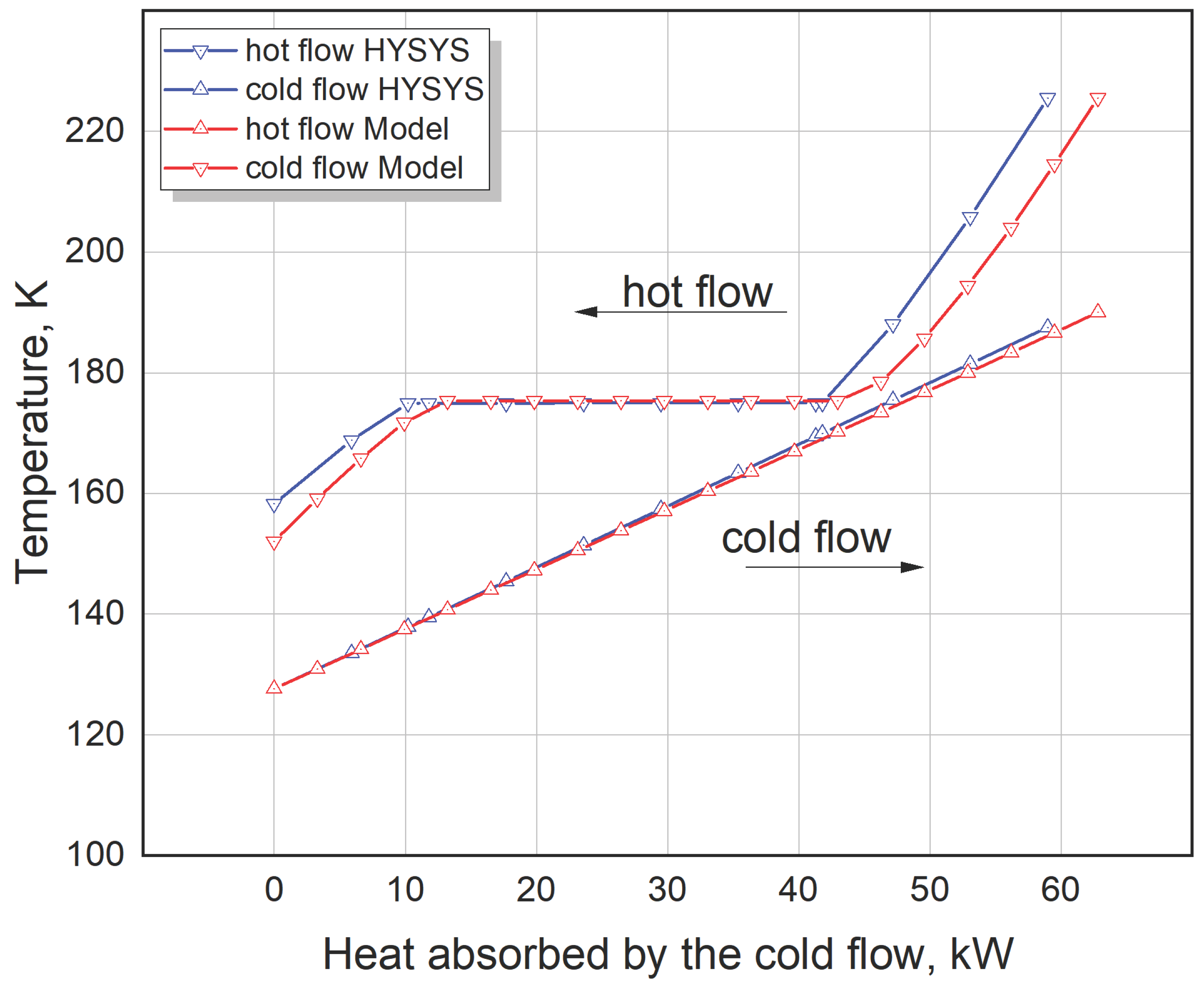
Figure 4.
T-h diagram of the CH4 - N2 - O2 mixture, where the composition matches that of the hot flow in the HEX (see Table 1).
Figure 4.
T-h diagram of the CH4 - N2 - O2 mixture, where the composition matches that of the hot flow in the HEX (see Table 1).

Figure 5.
The 3-flow MFHEX flows’ temperature with the heat transferred: simulated in the HYSYS AspenONE 12.1 program with given temperature difference at the MFHEX’s hot side: = 2.0, K; = 3.0, K.
Figure 5.
The 3-flow MFHEX flows’ temperature with the heat transferred: simulated in the HYSYS AspenONE 12.1 program with given temperature difference at the MFHEX’s hot side: = 2.0, K; = 3.0, K.

Figure 6.
The 3-flow MFHEX flows’ temperature with the cross-sectional indexes: simulated in the HYSYS AspenONE 12.1 program with given temperature difference at the MFHEX’s hot side: = 2.0, K; = 3.0, K.
Figure 6.
The 3-flow MFHEX flows’ temperature with the cross-sectional indexes: simulated in the HYSYS AspenONE 12.1 program with given temperature difference at the MFHEX’s hot side: = 2.0, K; = 3.0, K.

Figure 7.
Comparison of the 3-flow MFHEX flows’ temperature with the heat transferred: calculated in the program reported with , K, and simulated in the HYSYS AspenONE 12.1 program with = 12.69, K; = 9.12, K.
Figure 7.
Comparison of the 3-flow MFHEX flows’ temperature with the heat transferred: calculated in the program reported with , K, and simulated in the HYSYS AspenONE 12.1 program with = 12.69, K; = 9.12, K.

Figure 8.
Comparison of the 3-flow MFHEX flows’ temperature with the cross-sectional indexes: calculated in the program reported with , K, and simulated in the HYSYS AspenONE 12.1 program with = 12.69, K; = 9.12, K.
Figure 8.
Comparison of the 3-flow MFHEX flows’ temperature with the cross-sectional indexes: calculated in the program reported with , K, and simulated in the HYSYS AspenONE 12.1 program with = 12.69, K; = 9.12, K.


Table 1.
Initial data for calculating the Tq-diagram of the counterflow HEX.
| Flow | Working fluid | Flow parameters at the HEX’s inlet ports | ||||
|---|---|---|---|---|---|---|
| type | index | component | composition | Temperature | Pressure | Mass rate |
| mol/mol | K | bar | kg/h | |||
| Hot | 1 | CH4 | 99.973178 | 225.5 | 28.11 | 408.8680 |
| N2 | 0.024569 | |||||
| O2 | 0.002257 | |||||
| Cold | 1 | CH4 | 99.969465 | 127.6473 | 2.0 | 1677.9048 |
| N2 | 0.028048 | |||||
| O2 | 0.002490 | |||||
Table 2.
Results of the 2-flow HEX calculation based on (δε = 0.0001; ΔTas =5.0, K).
| ΔTmin | ε’ | Qact | Thot – Tcold | ||
|---|---|---|---|---|---|
| hot port | сold port | internal, min | |||
| K | W | K | |||
| 0.0 | 1.00 | 66992.8 | 31.3 | 14.9 | 0.0002 |
| 2.0 | 0.98 | 65324.1 | 32.9 | 18.8 | 2.0009 |
| 3.0 | 0.96 | 64490.4 | 33.8 | 20.6 | 3.0007 |
| 5.0 | 0.94 | 62820.6 | 35.5 | 24.4 | 5.0027 |
| 8.0 | 0.88 | 58627.4 | 39.7 | 33.3 | 8.0000 |
Table 3.
Results of the 2-flow HEX calculation in the HYSYS AspenONE 12.1 program.
| Thot – Tcold | Qact | ε’ | ||
|---|---|---|---|---|
| hot port | сold port | internal, min | ||
| K | W | |||
| 30.0 | 13.9 | -2.9 | 66820.0 | -- |
| 33.0 | 20.5 | 0.009 | 63880.0 | 1 |
| 35.0 | 24.7 | 2.0 | 61920.0 | 0.97 |
| 36.0 | 26.7 | 3.0 | 60940.0 | 0.95 |
| 38.0 | 30.6 | 5.0 | 58980.0 | 0.92 |
Table 4.
Initial data for calculating the Tq-diagram of the 3-flow MFHEX.
| Flow | Working fluid | MFHEX flows inlet parameters | ||||
|---|---|---|---|---|---|---|
| type | index | component name | composition | temperature | pressure | mass rate |
| mol/mol | K | bar | kg/h | |||
| Hot | 1 | N2 | 78.11 | 303.0 | 38.80 | 3292.0 |
| O2 | 20.96 | |||||
| Ar | 0.93 | |||||
| Cold | 1 | N2 | 62.21 | 104.8 | 1.50 | 1950.0 |
| O2 | 36.18 | |||||
| Ar | 1.61 | |||||
| 2 | N2 | 1.0 | 160.0 | 1.50 | 1091.0 | |
Table 5.
Results of the 3-flow MFHEX (see Table 4) calculation based on (δε = 0.0001; ΔTas =10.0, K); objective function , (39).
Table 5.
Results of the 3-flow MFHEX (see Table 4) calculation based on (δε = 0.0001; ΔTas =10.0, K); objective function , (39).
| ΔTmin | ε’ | Qact | Thot – Tcold_2 | Thot – Tcold_1 | ||||
|---|---|---|---|---|---|---|---|---|
| cold port | hot port | internal, min/max/avr | cold port | hot port | internal, min/max/avr | |||
| K | kW | K | ||||||
| 0.0 | 1.00 | 147.069 | 5.03 | 4.12 | 0.001/5.03/1.67 | 60.23 | 5.73 | 5.73/60.23/30.28 |
| 2.0 | 0.98 | 144.965 | 6.55 | 6.11 | 2.00/6.55/3.60 | 61.75 | 8.50 | 8.50/61.75/32.59 |
| 3.0 | 0.97 | 143.908 | 7.31 | 7.11 | 3.01/7.31/4.57 | 62.51 | 9.89 | 9.89/62.51/33.76 |
| 5.0 | 0.96 | 141.781 | 8.96 | 9.12 | 5.00/9.12/6.53 | 64.16 | 12.69 | 12.69/64.16/36.11 |
| 8.0 | 0.94 | 138.547 | 11.52 | 12.18 | 8.00/12.18/9.52 | 66.72 | 16.95 | 16.95/66.72/39.69 |
Table 6.
Results of the 3-flow MFHEX calculation (see Table 4) in the HYSYS AspenONE 12.1 program: the temperature difference at the MFHEX hot port (Thot – Tcold [1]) and (Thot – Tcold[2]) are given.
| ΔTmin | ε’ | Qact | Thot – Tcold_2 | Thot – Tcold_1 | ||||
|---|---|---|---|---|---|---|---|---|
| cold port | hot port | internal, min/max/avr | cold port | hot port | internal, min/max/avr | |||
| K | kW | K | ||||||
| 0.10 | 1.0 | 145.300 | 5.70 | 3.00 | 0.1/5.7/1.75 | 60.90 | 4.00 | 4.0/60.9/29.64 |
| 1.31 | 0.99 | 144.026 | 6.68 | 4.12 | 1.31/6.68/2.88 | 61.88 | 5.73 | 5.73/61.88/31.09 |
| 3.34 | 0.98 | 141.925 | 8.32 | 6.11 | 3.34/8.32/4.83 | 63.52 | 8.50 | 8.5/63.52/33.43 |
| 4.35 | 0.97 | 140.871 | 9.15 | 7.11 | 4.35/9.15/5.81 | 64.35 | 9.89 | 9.89/64.35/34.61 |
| 6.39 | 0.95 | 138.750 | 10.84 | 9.12 | 6.39/10.84/7.78 | 66.04 | 12.69 | 12.69/88.04/36.99 |
| 9.51 | 0.93 | 135.524 | 13.44 | 12.18 | 9.51/13.44/10.79 | 68.64 | 16.95 | 16.95/68.64/40.61 |
Disclaimer/Publisher’s Note: The statements, opinions and data contained in all publications are solely those of the individual author(s) and contributor(s) and not of MDPI and/or the editor(s). MDPI and/or the editor(s) disclaim responsibility for any injury to people or property resulting from any ideas, methods, instructions or products referred to in the content. |
© 2025 by the authors. Licensee MDPI, Basel, Switzerland. This article is an open access article distributed under the terms and conditions of the Creative Commons Attribution (CC BY) license (http://creativecommons.org/licenses/by/4.0/).
Copyright: This open access article is published under a Creative Commons CC BY 4.0 license, which permit the free download, distribution, and reuse, provided that the author and preprint are cited in any reuse.