
Submitted:
02 November 2025
Posted:
04 November 2025
You are already at the latest version
Abstract
Mapping Plant Ecological Units (PEUs) supports sustainable rangeland management, yet distinguishing them from multispectral imagery remains challenging due to high intra-class variability and spectral overlap. This study evaluates the contribution of auxiliary data layers to improve PEU classification from Landsat-8 OLI imagery in semi-arid rangelands of northeastern Iran. A Random Forest (RF) classifier was trained using field samples and multiple feature combinations, including spectral indices, topographic variables (DEM, slope, aspect), and Principal Component Analysis (PCA) components. Classification performance was assessed using Overall Accuracy (OA), Kappa coefficient, and non-parametric Friedman and post-hoc tests to determine significant differences among scenarios. The results show that auxiliary features consistently enhanced classification performance compared with spectral bands alone. In particular, integrating DEM and PCA layers yielded the highest accuracy (OA = 79.3%, κ = 0.71), with statistically significant improvement (p < 0.05). The findings demonstrate that incorporating topographic and transformed spectral information can effectively reduce class confusion and improve the separability of PEUs in complex rangeland environments. The proposed workflow provides a transferable approach for ecological unit mapping in other semi-arid regions facing similar environmental and management challenges.
Keywords:
vegetation mapping
; auxiliary data
; random forest
; accuracy assessment
; plant ecological units
1. Introduction
Satellite images form the basis of land cover and vegetation mapping and monitoring, owing to the periodic and accurate data [1,2]. Land cover mapping using remote sensing and satellite imagery is used for monitoring and managing natural resources, vegetation, and landscapes, as well, assessing and quantifying ecosystem services [3,4,5,6,7]. Plant Ecological Units (PEUs) are defined as the potential vegetation communities occurring at a landscape or site that differ from other vegetated land covers in their potential to generate determined types and quantities of vegetation [8]. Therefore, PEUs provide a standard reference for monitoring and land management [9]. Even though the notion of PEUs in natural resource and land cover assessment and monitoring is commonly accepted [10], the application and importance of PEUs still need to be better understood. The identification of PEUs remains challenging in the landscape [11], despite five decades of application of satellite image processing and remote sensing (RS) for monitoring and mapping land cover and vegetation. In general, PEUs have a complex spatial structure and quite similar spectral behavior, which results in reduced separability and classification inter-class. [12]. Thus, these heterogeneous plant communities are challenging to classify using remote sensing satellite images [13]. Processing and classifying optical remote sensing imagery for trustworthy and accurate PEUs mapping in heterogeneous landscapes using merely reflectance satellite imagery (e.g., reflectance data) is difficult due to the similarity in spectral behavior of PEUs [14], more specifically in arid rangelands where soil background dominates reflectance from vegetation canopy cover [15].
In the literature, numerous methods have been presented to overcome the difficulty of distinguishing land cover features with overlapping spectral characteristics. Particularly, the incorporation of auxiliary geospatial data in addition to satellite reflectance imagery has been recommended to facilitate distinguishing land cover features from satellite data [6,16,17,18,19]. However, the choice of input data and auxiliary data to enhance the precision of land cover and vegetation classification is still a controversial topic [20]. Many types of auxiliary geospatial data can be potentially fused to improve and enhance land cover classification and mapping performance. Usual data sources include: (1) topographic data such as DEM (Digital Elevation Models), and (2) vegetation indices, owing to their potential to target specific land cover and vegetation classes. Also, (3) linear transformation techniques like PCA (Principal Component Analysis) and TCT (Tasselled cap transformation) proved to be efficient auxiliary data sources in increasing and enhancing land cover and vegetation mapping accuracy [21,22].
While the utilisation of complementary auxiliary data has been well established in increasing the classification accuracy of satellite images, the process of detecting and classifying vegetation types is more complex. Since PEUs are a subclass of grassland vegetation, they exhibit very similar spectral reflectance, which presents an intricate classification task, especially when Landsat OLI-8 data are used for mapping.
So far, the impact of complementary auxiliary datasets on the accuracy of PEUs classification for rangeland monitoring and assessment has yet to be quantitatively assessed, especially in arid lands. Therefore, in this study, we propose to bridge this science gap by investigating the impact of complementary auxiliary datasets on PEUs classification. We selected a heterogeneous landscape with four distinguishable and dominant PEUs as our study area. Therefore, this study focused on increasing the accuracy of mapping and classification of PEUs using geospatial auxiliary data derived from reflectance bands of the akin images or produced independently. As such, it brings us to the following main objective: to improve PEUs mapping using combinations of the following types of complementary auxiliary data: (1) spectral vegetation indices, (2) linear transformation methods, and (3) topographic factors of DEM in improving PEUs mapping to reveal their pros and cons.
2. Materials and Methods
2.1. Study Region
The study area is located in southwestern Iran (Figure 1). This landscape covers an area of 7736 ha with an average elevation of 2697 m a.s.l., expanding from 32°03’56” to 32°04’05” N and 51°18’53” to 51°19’12” E. Its climate is characterized by dry summers and cold, temperate winters; the average 50-year rainfall in this region is about 200 mm. Due to appropriate management strategies, harvesting intensity is low, and despite the low rainfall (200mm), this region has good conditions for plant growth, with shrubs and perennial grasses forming the dominant vegetation type [23].
2.2. Field Measurements of PEUs
Four PEU types, namely PEU 1 (As ve (Astragalus verus Olivier)), PEU 2 (Br to (Bromus tomentellus Boiss)), PEU 3 (Sc or (Scariola orientalis Sojak )), and PEU 4 (As ve- Br to (Astragalus verus Olivier-Bromus tomentellus Boiss), were identified in the region. Vegetation cover percentage data using the physiognomic-floristic classification method can be used to identify the PEUs’ dominant types. We identified four PEU types in the region and sampled each type using three replicates. In each PEU, the vegetation cover percentage was estimated along three 100 m transects. The sampling points were tried to have the same distribution in the region (Figure 1).
Alongside each transect, 30 quadrats were located, which are made of 360 sampling quadrats in total. The sampling was systematic-randomly done, i.e., the first node was selected systematically, but the others were randomly distributed along the transect. The vegetation percentage of each species was estimated in each square to discern PEUs’ composition. The attributes of the PEUs are displayed in Table 1.
2.3. Satellite Data
We first downloaded Landsat OLI-8 (Landsat Operational Land Imager). images acquired on June 10, 2018. Images downloaded from the USGS (https://earthexplorer.usgs.gov/). This date approaches the peak in the phenological and productivity development of the major PEUs in the region, which are critical for accurately classifying land-cover types. Bands from Landsat 8 that are Uninformative to the vegetation analysis (such as cirrus clouds, coastal aerosol, and thermal bands) were removed. All Landsat 8 bands were surface reflectance corrected by the USGS.
2.4. Methodology
2.4.1. Image’s Pan Sharpening
Spatial resolution of Landsat OLI-8 bands varies from 15 m (panchromatic band) to 30 m (multispectral bands). To exploit the robustness of the panchromatic band (having higher spatial resolution and a wider spectral wavelength) and, as a result, to increase the accuracy of the PAUs classification maps, the 30 m resolution bands (bands 2 to 7) were enhanced to 15m resolution using the panchromatic band (band 8).
2.4.2. Auxiliary Geospatial Data
The pan-sharpened bands (2–8 bands) were stacked into a set of reflection bands. Then, the following auxiliary geospatial data derived from reflectance bands were calculated and used as the auxiliary data next to the reflectance bands of Landsat-8 imagery:
- Vegetation indices of Modified Soil Adjusted Vegetation Index (MSAVI), as a representative of soil-adjusted vegetation indices.
- Enhanced Vegetation Index (EVI)
- Proportion Vegetation (PV), as well as three image transformation outcomes, namely
- Principal Component Analysis (PCAs)
- Tasseled Cap Transformation (TCT)
- Digital Elevation Model (DEM)
PCA analysis was performed to extract the first three principal components of the reflectance bands, PC1, PC2, and PC3. The PCA products were generated using spectral information and explain more than 99% of the information and data variation.
The Tasselled cap 3-dimensional transformation was applied to the six bands of OLI-8 data (2-8, excluding the thermal bands, Cirrus, and coastal bands) to merge spectral data into a few bands of greenness, brightness, and wetness with little loss of information. Greenness is determined by a high reflectance in the near-infrared band and a high absorption in visible bands, which considerably correlates with healthy biomass and leaf index [24]. Brightness is the weighted sum of all reflective bands, representing natural, artificial features, bare or semi-bare soil. Wetness is sensitive to plant and soil moisture [25]. The greenness, brightness, and wetness indices were calculated using Eqs. See Table 2.
Since topography influences the dispensation of many PEUs, a 15 m resolution DEM was used in the classification. The DEM data was extracted from the SRTM (Shuttle Radar Topographic Mission), 30 m DEM was then merely rescaled to 15*15 m to be used together with reflectance-pan-sharpened multispectral Landsat-8 OLI data. This rescaled DEM was added to the dataset for further analysis as auxiliary data. SRTM-DEM data are available freely at USGS. Details of the auxiliary dataset used to increase the PEUs’ maps’ accuracy are presented in Table 2.
2.4.3. Sampling PEUs
After the field survey and the introduction of four dominant PEUs groups in the area, a total of 300 geographic (XY) locations were recorded using a handheld GPS for four PEUs (Figure 1c). The sampling points were distributed into two groups: “training points” to be classified (60%) and “test points” to validate the classification results (40%) [26].
2.4.4. PEUs Mapping Using Reflectance Bands and Auxiliary Data
We first classified pan-sharpened reflectance bands of Landsat OLI-8 images based on training sample sites (points). Then, to reveal the determine of auxiliary data on enhancing the accuracy of PEU mapping, each auxiliary band was added to the classification multispectral bands separately, and the images were reclassified using the same field-gathered training data used in the previous phase to avoid sampling effects.
The Classification Random Forest (RF) algorithm [27,28] was applied for the classification of PEUs after testing different classification algorithms (MaxLike, MinDist, neural network, and RF).
The increase in PEU map accuracy was evaluated at the end of each classification process using the confusion matrix then estimated OA (Overall Accuracy), OK (Overall Kappa), UA (User’s Accuracy), and PA (Producer’s Accuracy). The users’ and producers’ accuracies of each PEU class were measured to determine the best classification accuracy after applying different auxiliary data. The equations used to calculate the OA (1), OK (2), UA (3), and PA (4) are given as follows:
Where n is the total number of all classifications; X ij, is an element, located at the ith row and jth column of the confusion matrix; UAi represents UA of class i, and PAj represents UA of class j.
2.4.5. Statistical Analysis of Adding Values of Multiple Auxiliary Data
To display the efficiency of the added values of auxiliary data on the PEUs mapping accuracy of reflectance bands, in addition to the customary values of OA and OK index, we used the Friedman test with the post-hoc comparison of means following Demsar [29]. This test measures different PEUs in terms of UA, PA, and KIA (Kappa index of agreement) values, which were regarded as repeated measures over multiple data sets used for classification.
Figure 2 shows the methodology applied in this study to evaluate the result of different auxiliary datasets on PEUs’ mapping accuracy. First, the 30m bands (2-7) were pan-sharpened using the 15 m panchromatic band (band 8) of the OLI-8 sensor. Then, the complementary auxiliary layers of MSAVI, EVI, PV, and PCAs, TCT derived from reflectance bands, and DEM were used to develop collection datasets to enhance the PEUs mapping accuracy. The collected point samples were divided into training points (60%) for classification and test points (40%) for accuracy assessment. Following, the resulting map from the classification of reflectance bands, and reflectance bands complemented with each auxiliary data, were validated using test points. Finally, a statistical comparison was performed to reveal each auxiliary data point, adding values to the classification of reflectance bands.
3. Results
3.1. Reflectance Bands and Auxiliary Data Used for Classification
Figure 3 shows the auxiliary datasets used to enhance the PEUs’ mapping accuracy. These data include a false color-composite of Landsat OLI-8 ( bands 3 (green), 4 (red), 5 (near-infrared)), EVI, MSAVI, PV, TASSCAP-wetness (TC-W), PCAs, all derived from Landsat 8-OLI data, as well as rescaled to 15*15 m DEM.
3.2. Impact of Auxiliary Data on PEU Classification Accuracy
Confusion matrix results for the accuracy evaluation of PEU classification achieved from crossing testing points with the resulting map of classification datasets of reflectance bands and auxiliary data, are presented in Table 3. As displayed in this table, UA, PA, and KIA for each PEUs, moreover OA and OK of each classification process, are shown. The results show that since pan-sharpened reflectance bands were applied, PEU1 had the highest PA (78%), UA (88%), and KIA (71%). However, PEU3 had the lowest PA (56%), UA (56%), and KIA (40%). The OK was 52 and the OA 65%. Adding the auxiliary data to the reflectance bands led to an enhancement in the classification accuracy. The auxiliary data effect showed that PCAs-DEM returned the highest OK (71%) and OA (79%). PEU1 had the highest PA (87%), UA (90%), and KIA (82%), and PEU4 had the lowest PA (69%), UA (74%), and KIA (58%), while PCA-DEM auxiliary data together with reflectance bands were used for classification. PEU1 had the highest PA, UA, and KIA in almost all auxiliary data, but in contrast, PEU4 had the lowest PA, UA, and KIA.
The effects of different auxiliary data on the OLA 8 images bands, to enhance PEUs classification accuracy, are presented in Figure 4. As indicated in Figure 4a, most of the PEUs’ classification maps benefit from auxiliary data up to 29%; however, some are negatively affected by up to 7%. PEU3 significantly benefits from all the auxiliary data in terms of PA, but MSAVI and PV negatively affect the classification accuracy of PEU2 by 7%. Likewise, PV, TS-W, and PCA also negatively affect the PA of PEU4 by up to 6%. PEU1 was neutral to some auxiliary data but profited from most of the auxiliary data in terms of PA, up to 11%. PEU2, PEU4, and PEU3 identification benefit from adding auxiliary data to the reflectance bands when PA is concerned.
As shown in Figure 4b, all but PEU1 significantly benefit from the auxiliary data, up to 21% in terms of UA. PEU3 and PEU2 significantly benefit from all the auxiliary data. Most of the auxiliary data negatively affect UA of PEU1 up to 11%, except PCAs-DEM, which positively affects UA by 2%. Likewise, PEU4 was affected slightly negatively by EVI (1%).
As indicated in Figure 4c, most PEU classification improves their KIA accuracy up to 35% from auxiliary data however, some were negatively affected up to 6%. Meanwhile, PEU3 benefits remarkably from all the auxiliary data. MASVI and PV negatively affect the KIA of PEU1 by 1% and PEU2 up to 6%. Likewise, PEU4 was negatively affected by PV and TC-W (up to 3%). The side-by-side comparison of the efficiency of reflectance pan-sharpened bands and auxiliary data showed that auxiliary data enhanced OA between 1–14% (Figure 4d) and OK between 2–19% (Figure 4e). Among the PEUs classification maps, the map resulting from PCAs-DEM resulted in the highest overall classification accuracy (14%) and OK accuracy (19%).
Figure 5 illustrates the PEUs classification maps using the RF classifier based on pan-sharpened bands and auxiliary data such as vegetation indices (EVI, MSAVI, PV), image transformation outcomes (TC-W, PCAs) and the topographic factor of DEM. In each of these maps, the spatial distribution of the PEUs appears relatively similar. PEU2 is mostly distributed in the central flat areas of the study area, while PEU1 and PEU4 are distributed in the steeply sloping areas where the altitude is higher (see DEM in Figure 3). PEU3 is distributed throughout almost the entire study area.
Figure 6 illustrates the resulting map from reflectance bands and auxiliary data of PCAs-DEM that indicated the highest OK (71%) and OA (79%). In this map, PEU4 comprises Shrub-Tall grass dominant species that cover about 44% of the area. In contrast, PEU3 is a dominant semi-shrub that occupies a small area (16%), PEU2 is a tall grass species, and PEU1 is a scrubby species that accounted for 18% and 20%, respectively.
3.3. Statistical Comparison
The UA, PA, and KIA for PEU classes were calculated and compared by Friedmans’ test with the corresponding post-hoc (Table 4) to reveal the added value of the auxiliary data on PEU classes. The results of auxiliary data comparison by Friedmans’ test indicated that the PCAs-DEM and DEM displayed statistically significant effects on PEUs classification (P < 0.05), but vegetation indices and tasselled-cap transformation did not show a significant added value to the reflectance data for PEUs classification (Table 4).
4. Discussion
Although traditional and field-based mapping approaches have proven to deliver high accuracy, the costs and time associated with producing such maps reduce their application. This study examined whether the pan-sharpened bands alongside auxiliary datasets are adequate to classify PEUs across heterogeneous rangelands. In this study, the PEUs’ classification is based on the premise that each PEU class results from a distinct combination of dominant species and environmental ecological effects applied to distinguish the PEU classes. Four PEU types, namely PEU 1 (As ve (Astragalus verus Olivier)), PEU 2 (Br to (Bromus tomentellus Boiss)), PEU 3 (Sc or (Scariola orientalis Sojak )), and PEU 4 (As ve- Br to (Astragalus verus Olivier_ Bromus tomentellus Boiss), were identified in the region.
We used Landsat OLI 8 images in this study. Although these sensor images, due to their high spatial and temporal resolution, have demonstrated their utility for land use and land cover mapping [30]. However, the PEU’s classification is more complicated due to the similar spectral behavior of PEUs and the intricate spatial structure of the landscape. Nevertheless, 30 m spatial resolution bands likely lead to complex pixels and consequently low classification maps precision, especially at the subclass of plant community, i.e., PEUs. Thus, to circumvent the problem and reduce the mixed pixels effects, the 30 m resolution bands (bands 2 to 7) were pan-sharpened using the panchromatic band with a 15m resolution (band 8). A suite of classification algorithms has been explored for vegetation mapping. However, their success and efficiency depend on many factors, such as satellite images, the classification system, the characteristics of the study area, and the use of auxiliary datasets [31].
In this study, pan-sharpened Landsat OLI-8 images were classified using an RF algorithm. Such an approach will allow for improving PEUs classification with very fragmented, heterogeneous vegetation communities and spectrally similar features [30,32].
Lu et al. [33] in their research showed that in land cover mapping using spectral bands, the maximum likelihood classification (MLC) algorithm provides the most accurate maps compared to other classification algorithms and even machine learning algorithms. However, when additional auxiliary datasets were used, machine learning classifiers provided superior classification results than MLC. The RF algorithm relies on recursive sub-setting, which organizes the training data into groups of increasing homogeneity [27]. The relatively higher performance of the RF classifier suggests a level of intra-class variability, making recursive sub-setting efficient [34,35].
4.1. The Roles of Reflectance Bands and Auxiliary Dataset Features
We used two models for PEUs’ classification of arid rangelands. The first model includes only pan-sharpened bands (2-8 reflectance bands) from Landsat OLI-8 images. The overall classification accuracy (65%) and OK (52%) obtained in the first model (Table 3), indicated that the reflectance bands of Landsat OLI_8 images were still the most significant feature in PEUs classification. According to Table 3, PEU1 had the highest KIA (71%), but PEU3 had the lowest KIA (40%). PEU3 is usually characterized by a scattered and irregular distribution on the map, so that often between the PEUs visible large area of bare soil and bare space, ranging from a few square meters and in some cases, even several meters. Therefore, the presence of bare spaces and bare soil and their influence on the reflectance recorded by the sensors has probably reduced the PEUs map accuracy. Thereby, the distribution form of the PEUs may play a significant role in the intra-class spectral variation.
The second step is based on auxiliary data complementing the reflectance data. While the development of an auxiliary dataset is often time-consuming, it is the most effective way to identify and determine auxiliary datasets to improve the PEUs classification accuracy in heterogeneous landscapes. This research introduces an appropriate auxiliary dataset, including topographic data such as DEM, vegetation indices such as MSAVI, EVI, and PV, and linear transformation methods such as PCAs and TC-W, which are effective in enhancing PEUs mapping accuracy. The second step results showed that combinations of different auxiliary data could enhance OA and OK classification (1–14% and 2-19%, respectively). As opposed to using only reflectance bands, nearly all of the auxiliary data improved classification accuracy. As indicated in Figure 4d and e, among the auxiliary data, vegetation indices such as MSAVI, EVI, and PV have the least positive effect on classification precision. The vegetation indices are normally derived from red and infrared bands. These two bands are already exploited when reflectance data are used. Therefore, less improvement is observed in the classification accuracy when vegetation indices are applied.
In contrast to vegetation indices, the topographic factor (DEM) and linear transformation methods of reflectance bands, i.e., PCAs and TC-W, respectively, yielded the highest classification accuracy and made the most impact on the PEUs’ accurate identification. Since PEUs are distributed differently in the study area, therefore, topographic variable of DEM is a thematic map that significantly improved PEUs classification. Likewise, the purpose of PCA is dimension reduction by determining the effective information. Therefore, PC1, PC2 and PC3 contain the highest spectral information (more than 99%); these PCs reduce noise and therefore significantly improve the PEUs maps’ accuracy. The Tasseled cap transformation was also extracted from the six bands (2-7 bands) to consolidate spectral data into a few bands with little loss of information. While most vegetation indices are only a combination of the two red and infrared bands, they are also present in the tasseled cap transformation. This can be regarded as the reason for the higher classification accuracy increment of Tasseled-cap transformation when compared with vegetation indices.
Figure 4 a-c illustrate that PEU3 substantially profits from all the auxiliary data. The classification result based on the reflectance data and the combination of DEM-PCAs auxiliary data has enabled us to easily separate PEU3 from other PEUs, with the greatest gain in accuracy compared with reflectance bands (35%). It seems that these two data layers of the auxiliary data set (DEM-PCAs ) reduced the effects of bare soil reflectance, thus presenting purer pixels of this PEU.
Conversely, vegetation indices (e.g., MASVI and PV) negatively affect the classification accuracy of PEU2 and somewhat PEU4. The role of the PEUs’ phenology should also be noted. For instance, the growth season of PEUs with dominant grass species (Br to) grows earlier than that of PEUs in the study area, while the growth season of PEUs with dominant shrub species (e.g., As ve and Sc or) starts with a significant delay compared to other PEUs. In addition, due to a mild grazing of the study area, PEU2 is more even and uniform than the other PEUs (e.g., PEU1 and PEU3), making it more distinguishable in the images. Other PEUs are more variable in terms of canopy reflectance at the same time due to shrubby species dominance or compositional variation (i.e., PEU1, PEU3, and PEU4). Finally, the sensors record a combination of soil and vegetation reflectance, thus increasing the number of mixed pixels and error rate in these PEUs. This is why auxiliary data such as PCA and PCA-DEM have substantial impacts on PEU2 classification. PCA has affected to easily extracting land cover signatures, which helped to classify the different PEUs.
PEU4 consists of two dominant vegetation types of As ve and Br to, so that due to structure and life form differences having dissimilar spectral behavior, therefore consequently lower accuracies of the classification map. The tested vegetation indices cannot detect and eliminate these errors. While auxiliary data such as DEM and PCA-DEM have substantial impacts on the PEU4 Kappa index of agreement. As mentioned before, PEUs’ spatial distribution is different; therefore, topographic variables are features in improving PEUs classification. As shown in Figure 5 and Figure 6, PEU2 is dispersed mainly in the flat Plains, whereas PEU1 and PEU3 are distributed on steeper slopes. PEU4 is distributed evenly, almost throughout the entire area. Vegetation indices acted mostly neutrally, or even negatively in some cases, for the classification of PEU1. Therefore, as much as the PEU1 is a concern due to its dense canopy cover and consequently delivering pure pixels, using vegetation indices as auxiliary data is not necessary. Yet, some of the auxiliary data, such as DEM and PCAS-DEM, effectively improved the spatial distribution of PEU1 and increased the classification accuracy.
The produced PEUs classification maps were validated by ground truth data (test points), and assessed by computing OA and OK (Figure 6). Resulting PEUs classification maps from pan-sharpened bands and auxiliary data of PCAs-DEM produced the highest OA (79%) and OK (71%). According to the Land Use and Land Cover classification system with satellite images data developed by Anderson [36], nine main classes were identified, including: Built-up Lands or Urbans, Rangelands, Agricultures, Forests, Wetlands, Waters, Tundra, Barren Land and Perennial Snow. Moreover, for each of these major classes of land use and land cover, subclasses have been introduced. So far, most of the land cover mapping process has been implemented on the main land cover classes, e.g., Macintyre [37] with OA, 50–74%, Pflugmacher [38] with OA, 75.1%, Feng [19] with OA, 76%, Castillejo-Gonzalez) [35] with OA, 72%. However, this study focused on performing the classification process for subclasses of rangeland vegetation (plant ecological units). When a vegetation subclass map is concerned (i.e., PEUs), a more similar spectral (low inter-class separability) is expected with a more intricate spatial structure. Therefore, their separation is a difficult process, and the OA of 79% achieved in this study is sufficiently satisfactory.
5. Conclusions
Accurately delineating PEUs from medium-resolution multispectral imagery remains challenging due to spectral similarity among vegetation types and spatial heterogeneity in semi-arid landscapes. This study shows that augmenting pan-sharpened Landsat OLI-8 bands with carefully selected auxiliary data can substantially improve PEU classification. In particular, the combination of DEM-derived topographic information and PCA components yielded the most consistent gains when used with an RF classifier. These results underscore that feature design matters as much as the base imagery: not all auxiliary layers contribute equally, and some offer little or no benefit. As a practical recommendation, we advocate prioritizing terrain derivatives (elevation, slope, aspect) and low-dimensional spectral transforms (first PCs) before adding additional indices or ancillary layers. This work provides an operational pathway for PEU mapping in semi-arid rangelands and can inform ecological monitoring and management. Future research should assess temporal robustness, adopt spatially explicit validation, compare additional learners and feature-selection strategies, and evaluate transferability to other regions. Together, these steps will further strengthen the reliability and scalability of PEU maps derived from satellite RS.
Author Contributions
For Methodology, A.E. and M.A.; conceptualization, A.E. and M.A.; software, M.A.; validation, A.E.; investigation, M.A.; resources, M.A.; formal analysis, M.A.; data curation, A.E. and M.A.; writing—original draft preparation, M.A. and J.V.; writing—review and editing, A.E., J.V., A.A.N. and E.A.; supervision, A.E.; visualization, M.A. and A.E.; project administration, A.E.; funding acquisition: J.V. All authors have read and agreed to the published version of the manuscript.
Funding
This work was supported by Shahrekord University. J.V. was funded by the European Union (ERC, FLEXINEL, 101086622). Views and opinions expressed are however those of the author(s) only and do not necessarily reflect those of the European Union or the European Research Council. Neither the European Union nor the granting authority can be held responsible for them.
Data Availability Statement
Data supporting this study may be provided by the first author upon a reasonable request. The data are not publicly available due to the privacy of parts of the data.
Conflicts of Interest
The authors declare no conflict of interest.
References
- Zhang, C.; Harrison, P.A.; Pan, X.; Li, H.; Sargent, I.; Atkinson, P.M. . Scale Sequence Joint Deep Learning (SS-JDL) for land use and land cover classification. Remote Sensing of Environment. 2020, 237, 111593. [Google Scholar] [CrossRef]
- Naegeli de Torres, F.; Richter, R.; Vohland, M. A multisensoral approach for high-resolution land cover and pasture degradation mapping in the humid tropics: A case study of the fragmented landscape of Rio de Janeiro. International Journal of Applied Earth Observation and Geoinformation 2019, 78, 189–201. [Google Scholar] [CrossRef]
- Yu, L.; Fu, H.; Wu, B.; Clinton, N.; Gong, P. Exploring the Potential Role of Feature Selection in Global Land-Cover Mapping. International Journal of Remote Sensing 2016, 37, 5491. [Google Scholar] [CrossRef]
- Topaloglu, R.H.; Sertel, E.; Musaoglu, N. Assessment of Classification Accuracies of Sentinel-2 and Landsat-8 Data for Land Cover / Use Mapping. ISPRS 2016, 12–19. [Google Scholar] [CrossRef]
- Zhang, X.; Liu, L.; Wang, Y.; Hu, Y.; Zhang, B. A SPECLib-based operational classification approach: A preliminary test on China land cover mapping at 30 m. International Journal of Applied Earth Observation and Geoinformation 2018, 71, 83–94. [Google Scholar] [CrossRef]
- Hurskainen, P.; Adhikari, H.; Siljander, M.; Pellikka, P.K.E.; Hemp, A. Auxiliary datasets improve accuracy of object-based land use/land cover classification in heterogeneous savanna landscapes. Remote Sensing of Environment 2019, 233, 111354. [Google Scholar] [CrossRef]
- Macintyre, P.D.; van Niekerk, A.; Mucina, L. Efficacy of multi-season Sentinel-2 imagery for compositional vegetation classification. International Journal of Applied Earth Observation and Geoinformation 2020, 85, 101980. [Google Scholar] [CrossRef]
- Stam, Carson A. Using Biophysical Geospatial and Remotely Sensed Data to Classify Ecological Sites and States. All Graduate Theses and Dissertations, 2012. https://digitalcommons.usu.edu/etd/1389.
- Spiegal, S.; Bartolome, J.W.; White, M.D. Applying ecological site concepts to adaptive conservation management on an iconic Californian landscape. Rangelands 2016, 38, 365–370. [Google Scholar] [CrossRef]
- Brown, J.R.; Bestelmeyer, B.T. An Introduction to the Special Issue “Ecological Sites for Landscape Management. Rangelands 2016, 38, 311–312. [Google Scholar] [CrossRef]
- Blanco, P.D.; del Valle, H.F.; Bouza, P.J.; Metternicht, G.I.; Hardtke, L.A. Ecological site classification of semiarid rangelands: Synergistic use of Landsat and Hyperion imagery. International Journal of Applied Earth Observation and Geoinformation 2014, 29, 11–21. [Google Scholar] [CrossRef]
- Rodriguez-Galiano, V.; Chica-Olmo, M. Land cover change analysis of a Mediterranean area in Spain using different sources of data: Multi-seasonal Landsat images, land surface temperature, digital terrain models and texture. Applied Geography 2012, 35, 208–218. [Google Scholar] [CrossRef]
- Sluiter, R.; Pebesma, E.J. Comparing techniques for vegetation classification using multi- and hyperspectral images and ancillary environmental data. International Journal of Remote Sensing 2010, 31, 6143–6161. [Google Scholar] [CrossRef]
- Thakkar, A.K.; Desai, V.R.; Patel, A.; Potdar, M.B. Post-classification corrections in improving the classification of Land Use/Land Cover of arid region using RS and GIS: The case of Arjuni watershed, Gujarat, India. The Egyptian Journal of Remote Sensing and Space Science 2017, 20, 79–89. [Google Scholar] [CrossRef]
- Aghababaei, M.; Ebrahimi, A.; Naghipour, A.A.; Asadi, E.; Verrelst, J. Monitoring of Plant Ecological Units Cover Dynamics in a Semiarid Landscape from Past to Future Using Multi-Layer Perceptron and Markov Chain Model. Remote Sens 2024, 16, 9–1612. (In Persian) [Google Scholar] [CrossRef]
- Rogan, J.; Miller, J.; Stow, D.; Franklin, J.; Levien, L.; Fischer, C. Land-cover change monitoring with classification trees using Landsat TM and ancillary data. Photogrammetric Eng. Remote Sens. 2003, 69, 793–804. [Google Scholar] [CrossRef]
- Ozdogan, M.; Gutman, G. A new methodology to map irrigated areas using multi-temporal MODIS and ancillary data: an application example in the continental US. Remote Sens. Environ. 2008, 112, 3520–3537. [Google Scholar] [CrossRef]
- Corcoran, J.M.; Knight, J.F.; Gallant, A.L. Influence of multi-source and multitemporal remotely sensed and ancillary data on the accuracy of random forest classification of wetlands in Northern Minnesota. Remote Sens. 2013, 5, 3212–3238. [Google Scholar] [CrossRef]
- Feng, D.; Yu, L.; Zhao, Y.; Cheng, Y.; Xu,Y. ; Li, C.; Gong, P. A multiple dataset approach for 30-m resolution land cover mapping: a case study of continental Africa. International Journal of Remote Sensing 2018, 39, 3926–3938. [Google Scholar] [CrossRef]
- Zhu, Z.; Gallant, A.L.; Woodcock, C.E.; Pengra, B.P.; Olofsson, T.; Loveland, R.; Jin, S.; Dahal, D.; Yang, L.; Auch, R.F. Optimizing selection of training and auxiliary data for operational land cover classification for the LCMAP initiative. ISPRS Journal of Photogrammetry and Remote Sensing 2016, 122, 206–221. [Google Scholar] [CrossRef]
- Lu, D.; Weng, Q. A survey of image classification methods and techniques for improving classification performance. International Journal of Remote Sensing 2007, 28, 823–870. [Google Scholar] [CrossRef]
- Khatami, R.; Mountrakis, G.; Stehman, S.V. A meta-analysis of remote sensing research on supervised pixel-based land-cover image classification processes: General guidelines for practitioners and future research. Remote Sensing of Environment 2016, 177, 89–100. [Google Scholar] [CrossRef]
- Aghababaei, M.; Ebrahimi, A.; Naghipour, A.A.; Asadi, E.; Verrelst, J. Vegetation Types Mapping Using Multi-Temporal Landsat Images in the Google Earth Engine Platform. Remote Sens 2021, 13, 22–4683. [Google Scholar] [CrossRef] [PubMed]
- Wang, D.; Wan, B.; Qiu, P.; Su, Y.; Guo, Q.; Wu, X. Artificial Mangrove Species Mapping Using Pléiades-1: An Evaluation of Pixel-Based and Object-Based Classifications with Selected Machine Learning Algorithms. Remote Sensing 2018, 10, 294. [Google Scholar] [CrossRef]
- Baig, M.H.A.; Zhang, L.; Shuai, T.; Tong, Q. Derivation of a tasselled cap transformation based on Landsat 8 at-satellite reflectance. Remote Sensing Letters 2014, 5, 423–431. [Google Scholar] [CrossRef]
- Aghababaei, M.; Ebrahimi, A.; Naghipour, A.A.; Asadi, E.; Verrelst, J. Classification of Plant Ecological Units in Heterogeneous Semi-Steppe Rangelands: Performance Assessment of Four Classification Algorithms. Remote Sens 2021, 13, 3433. (in Persian). [Google Scholar] [CrossRef]
- Aghababaei, M.; Ebrahimi, A.; Naghipour, A.A.; Asadi, E.; Perez-Suay, A.; Morata, M.; Garcia, J.L.; Rivera Caicedo, J.P.; Verrelst, J. Introducing ARTMO’s Machine-Learning Classification Algorithms Toolbox: Application to Plant-Type Detection in a Semi-Steppe Iranian Landscape. Remote Sens 2022, 14, 18–4452. [Google Scholar] [CrossRef]
- Punia, M.; Joshi, P. K.; Porwal, M.C. Decision tree classification of land use land cover for Delhi, India using IRS-P6 AWiFS data; Expert Syst. Appl 2011, 38, 5577–5583. [Google Scholar] [CrossRef]
- Demsar, J. Statistical Comparisons of Classifiers over Multiple Data Sets. Journal of Machine Learning Research 2006, 7, 1–30. [Google Scholar]
- Ouzemou, J.E.; Harti, A.; Lhissou, R.; Moujahid, A.; Bouch, N.; Ouazzani, R.; Bachaoui, M.; Ghmari, A. Crop type mapping from pansharpened Landsat 8 NDVI data: A case of a highly fragmented and intensive agricultural system. Remote Sensing Applications: Society and Environment 2018, 49–103. [Google Scholar] [CrossRef]
- Xie, Z.; Chen,Y. ; Lu, D.; Guiying, L.; Chen, E. Classification of Land Cover, Forest, and Tree Species Classes with ZiYuan-3 Multispectral and Stereo Data. Remote Sensing 2019, 11, 164. [Google Scholar] [CrossRef]
- Phiri, D.; Morgenroth, J.; Xu, C.; Hermosilla, T. Effects of pre-processing methods on Landsat OLI-8 land cover classification using OBIA and random forests classifier. International Journal of Applied Earth Observation and Geoinformation 2018, 73, 170–178. [Google Scholar] [CrossRef]
- Lu, D.; Li, G.; Moran, E.; Kuang, W. A comparative analysis of approaches for successional vegetation classification in the Brazilian Amazon. Gisci. Remote Sens 2014, 51, 695–709. [Google Scholar] [CrossRef]
- Rogan, J.; Franklin, J.; Stow, D.; Miller, J.; Woodcock, C.; Roberts, D. Mapping land-cover modifications over large areas: A comparison of machine learning algorithms. Remote Sens. Environ 2008, 112, 2272–2283. [Google Scholar] [CrossRef]
- Castillejo-Gonzalez, I.; Angueira, C.; Garcia-Ferrer, A.; Sanchez de la Orden, M. Combining Object-Based Image Analysis with Topographic Data for Landform Mapping: A Case Study in the Semi-Arid Chaco Ecosystem, Argentina. ISPRS International Journal of Geo-Information 2019, 8, 132. [Google Scholar] [CrossRef]
- Anderson, J.; Hardy, E.; Roach, J.; Witmer, R.E. A Land Use and Land Cover Classification System for Use with Remote Sensor Data. Geological Survey Professional, 1976, 964, U.S. Government Printing Office, Washington DC, 28.
- Macintyre, P.D.; Van Niekerk, A.; Dobrowolski, M.P.; Tsakalos, J.L.; Mucina, L. Impact of ecological redundancy on the performance of machine learning classifiers in vegetation mapping. Ecol Evol 2018, 8, 6728–6737. [Google Scholar] [CrossRef]
- Pflugmacher, D.; Rabe, A.; Peters, M.; Hostert, P. Mapping pan-European land cover using Landsat spectral-temporal metrics and the European LUCAS survey. Remote Sensing of Environment 2019, 221, 583–595. [Google Scholar] [CrossRef]
Figure 1.
The position of the region: (a - On the Iran border; (b)- on the province border; (c)- Study area border (Marjan). A set of recorded points from PEU that divided into two groups: training data (60%) for classifying PEU and testing data (40%) for evaluating of PEU classified maps.
Figure 1.
The position of the region: (a - On the Iran border; (b)- on the province border; (c)- Study area border (Marjan). A set of recorded points from PEU that divided into two groups: training data (60%) for classifying PEU and testing data (40%) for evaluating of PEU classified maps.
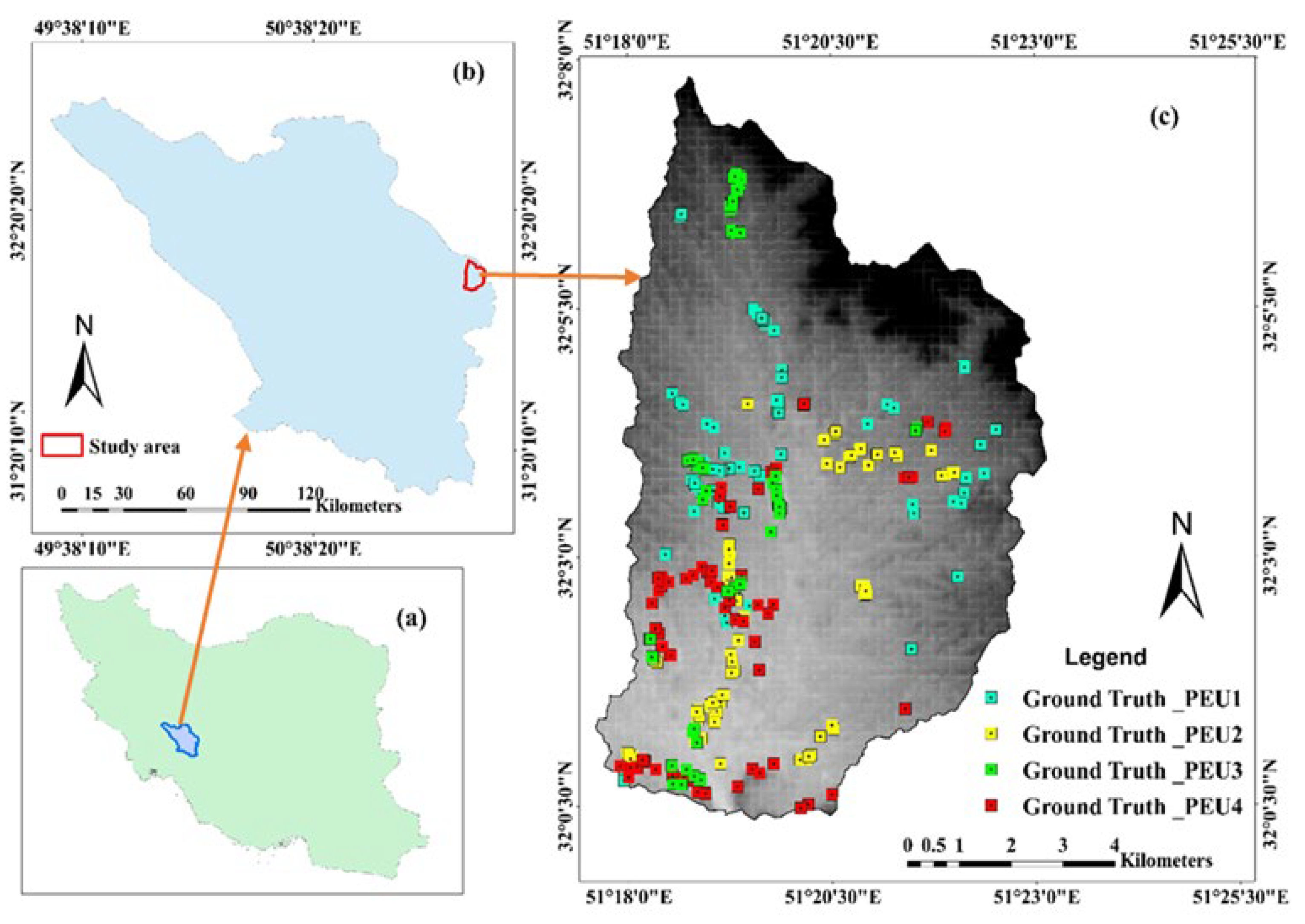
Figure 2.
The framework of mapping PEUs using reflectance bands of Landsat-8 OLI data and auxiliary data to enhance mapping accuracy in this study.
Figure 2.
The framework of mapping PEUs using reflectance bands of Landsat-8 OLI data and auxiliary data to enhance mapping accuracy in this study.
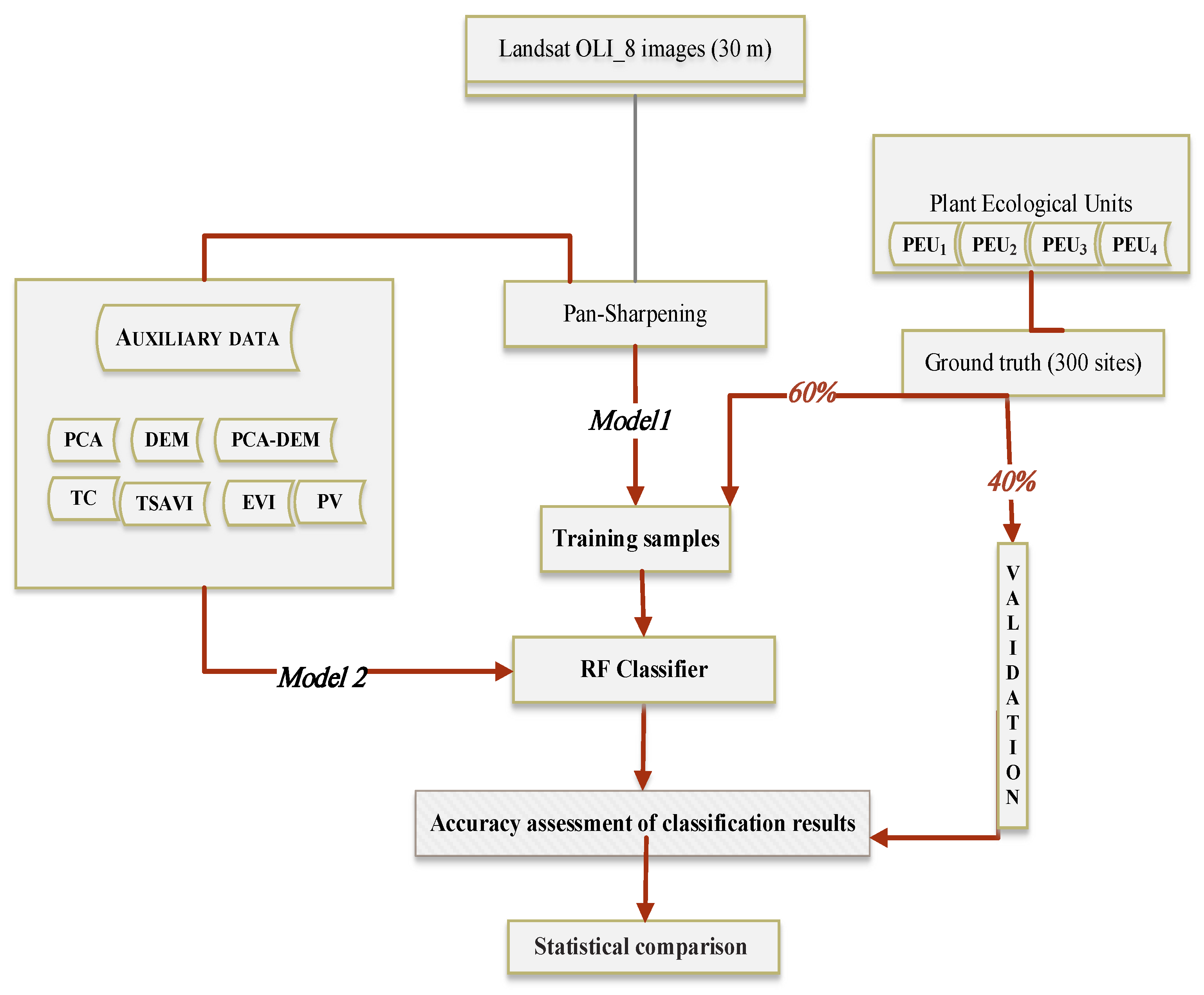
Figure 3.
Auxiliary dataset used to enhance the PEUs classification accuracy.
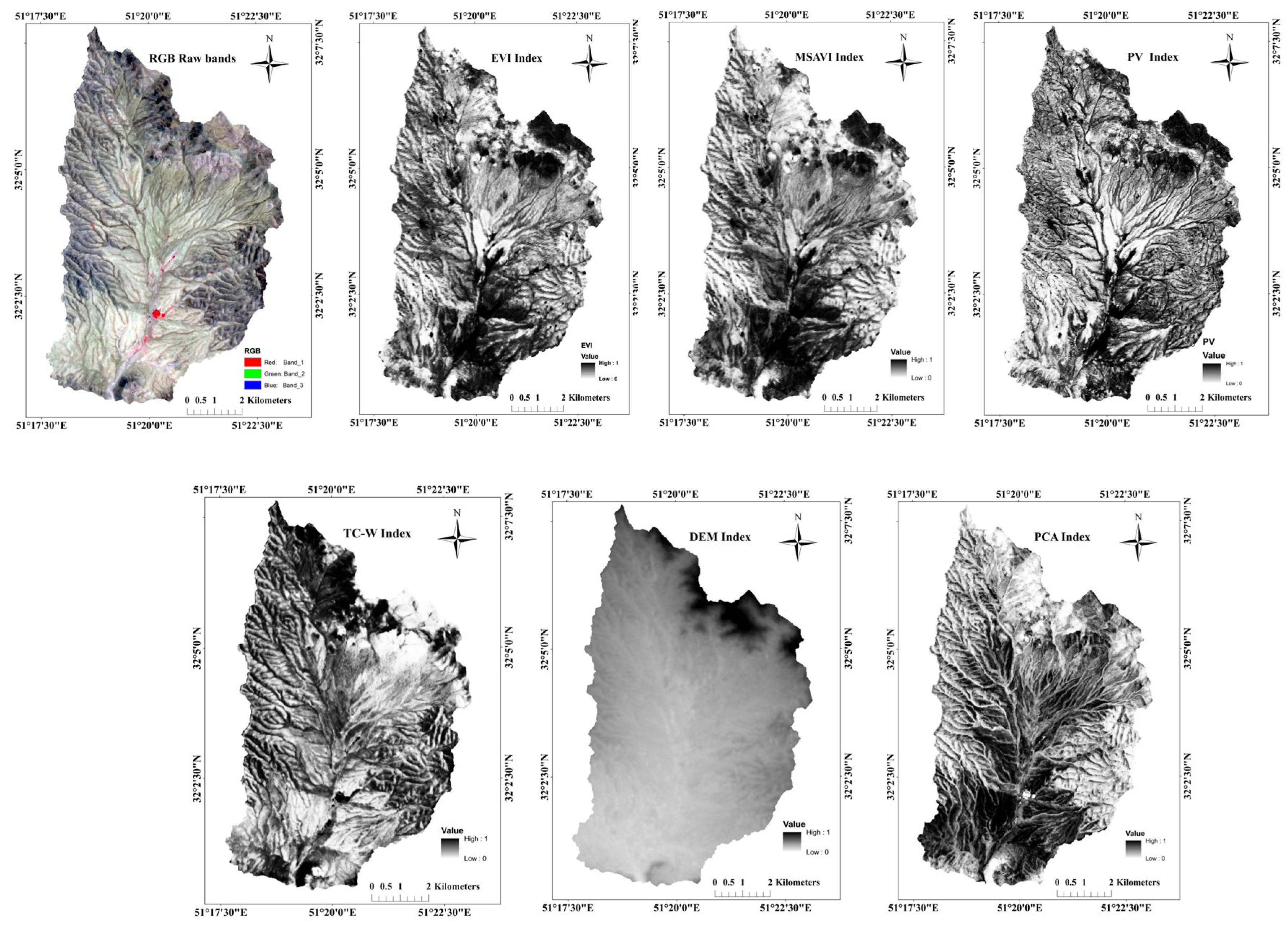
Figure 4.
Effects of different auxiliary data on the PEUs classification accuracy. a: UA b: PA, c: KIA: d: OA and e: OK.
Figure 4.
Effects of different auxiliary data on the PEUs classification accuracy. a: UA b: PA, c: KIA: d: OA and e: OK.
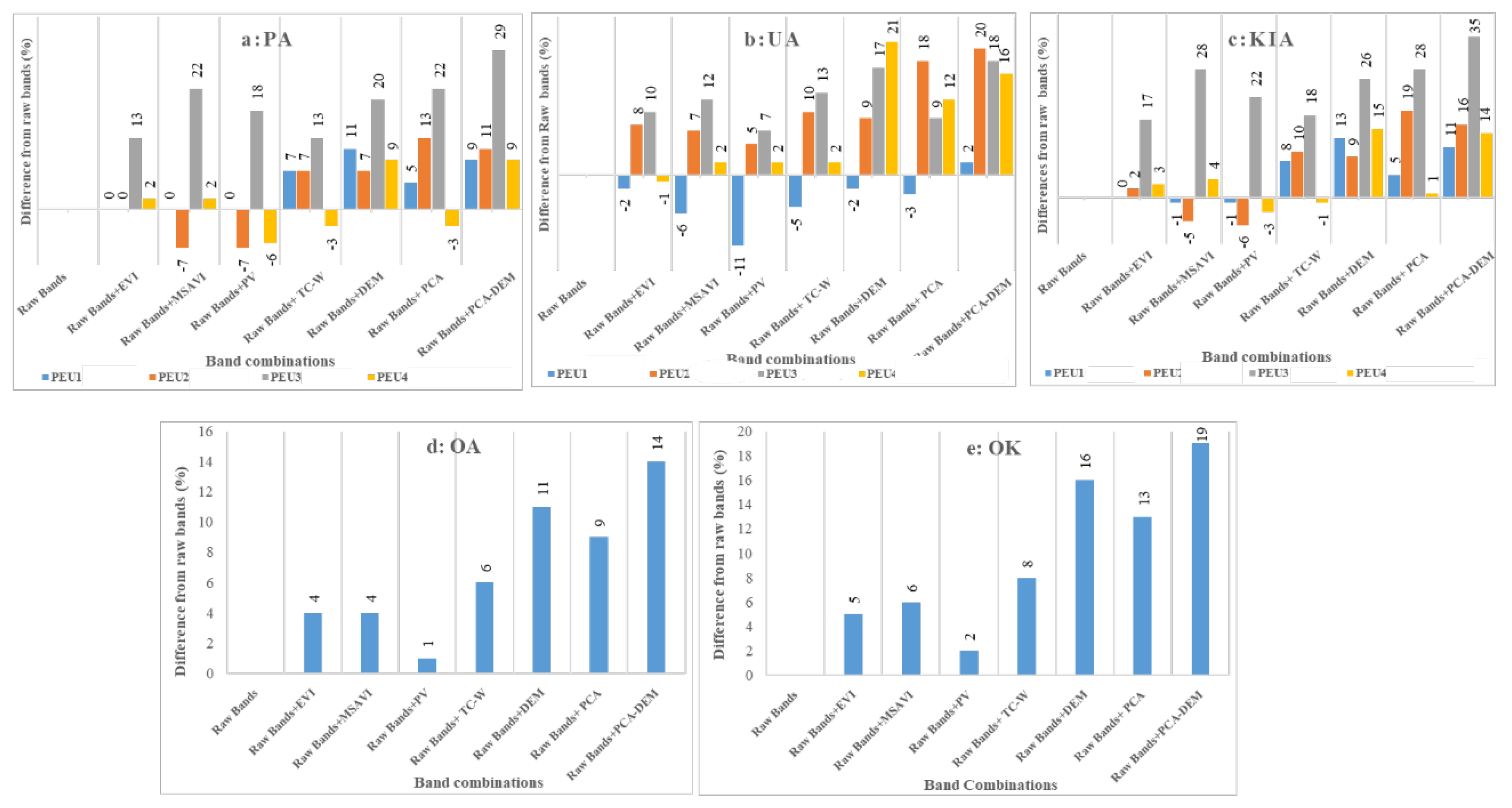
Figure 5.
PEUs classification maps using reflectance bands and complementary auxiliary datasets (EVI, MSAVI, PV, TC-W, PCAs and DEM).
Figure 5.
PEUs classification maps using reflectance bands and complementary auxiliary datasets (EVI, MSAVI, PV, TC-W, PCAs and DEM).
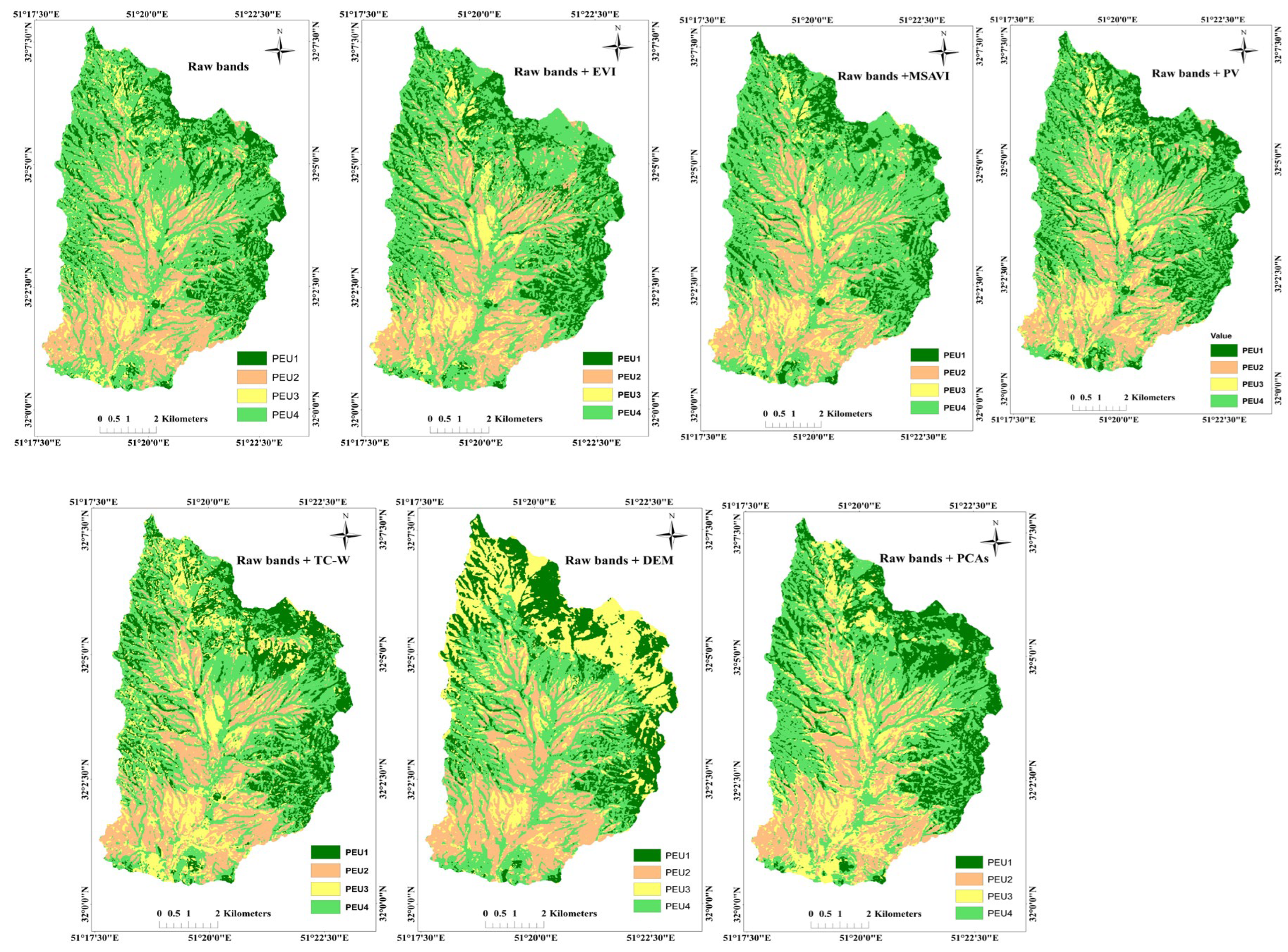
Figure 6.
The PEUs mapping resulting from pan-sharpened bands and PCAs-DEM as auxiliary data, which revealed the highest OK accuracy (71%) and OA (79%).
Figure 6.
The PEUs mapping resulting from pan-sharpened bands and PCAs-DEM as auxiliary data, which revealed the highest OK accuracy (71%) and OA (79%).
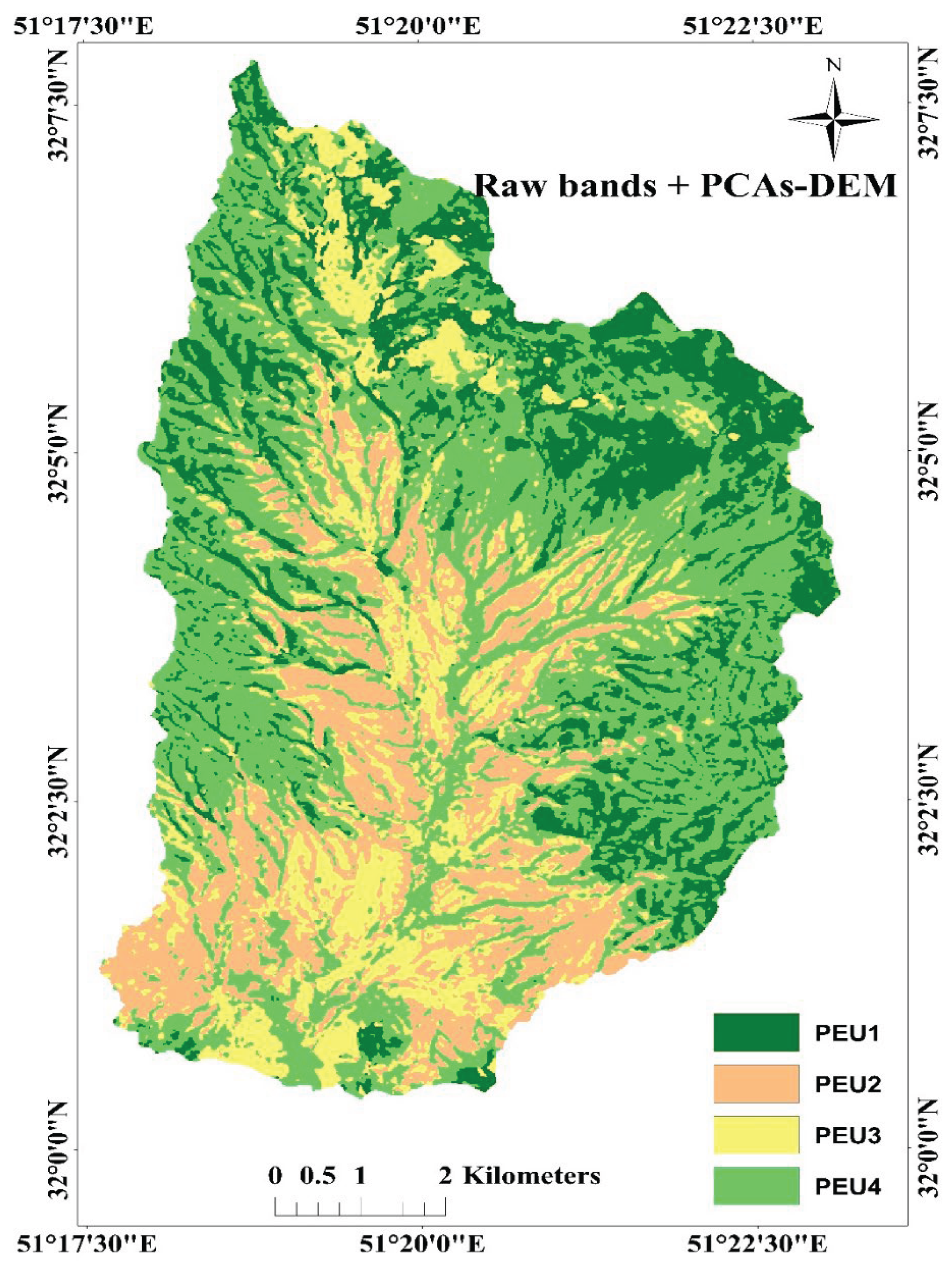

Table 1.
Selected PEUs and their vegetation characteristics in the region.
| Code | Field photos | Abbreviation | life-form |
|---|---|---|---|
| PEU 1 | 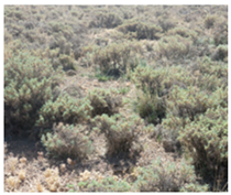 |
As ve | Shrub |
| PEU 2 | 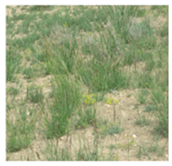 |
Br to | Tall grass |
| PEU 3 | 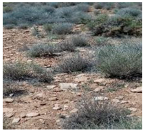 |
Sc or | Semi-shrub |
| PEU 4 | 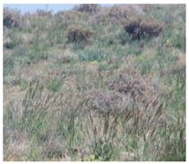 |
As ve-Br to | Shrub -Tall grass |
Table 2.
Specifications of Auxiliary dataset features used for PEU mapping.
| Auxiliary data | Formula/Description |
|---|---|
| Principal Component Analysis (PCAs) | This transformation technique is often used for data compression or noise removal |
| Digital Elevation Model (DEM) | 3D Cartographic ground representation of the terrain’s surface is the most common basis for digitally produced relief maps |
| Tasseled Cap-Wetness (TC-W) | OLI Wet = (OLI2*0.1511) + (OLI 3*0.1973) + (OLI4 *0.3283) + (OLI5 *0.3407) + (OLI6 *(-0.7117)) + (OLI7 *(-0.4559)) |
| Modified Soil-Adjusted Vegetation Index (MSAVI) | MSAVI=(NIR-RED)(1+L)/NIR+RED+L |
| Enhanced Vegetation Index (EVI) | EVI=2.5*(NIR-RED)/(NIR+6 * RED-7.5* Blue +1) |
| proportion vegetation (PV) | NDVI-NDVI (Min) / NDVI (Max) – NDVI(Min) |
Table 3.
Error matrix results table. Summary of the best PEUs classification accuracy by different auxiliary data.
Table 3.
Error matrix results table. Summary of the best PEUs classification accuracy by different auxiliary data.
| Reflectance Bands | Reflectance Bands + EVI | ||||||||
| PA | UA | KIA | PA | UA | KIA | ||||
| PEU1 | 78 | 88 | 71 | PEU1 | 78 | 86 | 71 | ||
| PEU2 | 65 | 60 | 51 | PEU2 | 65 | 68 | 53 | ||
| PEU3 | 56 | 56 | 40 | PEU3 | 69 | 66 | 57 | ||
| PEU4 | 60 | 58 | 44 | PEU4 | 62 | 57 | 47 | ||
| Overall Kappa: 52% Overall Accuracy: 65% | Overall Kappa: 57% Overall Accuracy: 69% | ||||||||
| Reflectance Bands + MSAVI | Reflectance Bands + PV | ||||||||
| PA | UA | KIA | PA | UA | KIA | ||||
| PEU1 | 78 | 82 | 70 | PEU1 | 78 | 77 | 70 | ||
| PEU2 | 58 | 67 | 46 | PEU2 | 58 | 65 | 45 | ||
| PEU3 | 78 | 68 | 68 | PEU3 | 74 | 63 | 62 | ||
| PEU4 | 62 | 60 | 48 | PEU4 | 54 | 60 | 41 | ||
| Overall Kappa: 58% Overall Accuracy: 69% | Overall Kappa: 54% Overall Accuracy: 66% | ||||||||
| Reflectance Bands + TC-W | Reflectance Bands + PCAs | ||||||||
| PA | UA | KIA | PA | UA | KIA | ||||
| PEU1 | 85 | 83 | 79 | PEU1 | 83 | 85 | 76 | ||
| PEU2 | 72 | 70 | 61 | PEU2 | 78 | 78 | 70 | ||
| PEU3 | 69 | 69 | 58 | PEU3 | 78 | 65 | 68 | ||
| PEU4 | 57 | 60 | 43 | PEU4 | 57 | 70 | 45 | ||
| Overall Kappa: 60% Overall Accuracy: 71% | Overall Kappa: 65% Overall Accuracy: 74% | ||||||||
| Reflectance Bands +DEM | Reflectance Bands + PCAs -DEM | ||||||||
| PA | UA | KIA | PA | UA | KIA | ||||
| PEU1 | 89 | 86 | 84 | PEU1 | 87 | 90 | 82 | ||
| PEU2 | 72 | 69 | 60 | PEU2 | 76 | 80 | 67 | ||
| PEU3 | 76 | 73 | 66 | PEU3 | 85 | 74 | 75 | ||
| PEU4 | 69 | 79 | 59 | PEU4 | 69 | 74 | 58 | ||
| Overall Kappa: 68% Overall Accuracy: 76% | Overall Kappa: 71% Overall Accuracy: 79% | ||||||||
Table 4.
Results of statistically significant comparison (P<0.05) between the accuracy of PEUs and auxiliary data.
Table 4.
Results of statistically significant comparison (P<0.05) between the accuracy of PEUs and auxiliary data.
| PEUs Accuracy | Sig | Auxiliary dataset Accuracy | Sig |
|---|---|---|---|
| UA | 0.021* | Reflectance bands-EVI | .613 |
| Reflectance bands-MSAVI | .665 | ||
| Reflectance bands-PV | .773 | ||
| Reflectance bands-TC-W | .248 | ||
| Reflectance bands- PCAs | .194 | ||
| Reflectance bands-DEM | 0.036* | ||
| Reflectance bands- PCAs -DEM | 0.004* | ||
| PA | 0.025* | Reflectance bands-EVI | .665 |
| Reflectance bands-MSAVI | .470 | ||
| Reflectance bands-PV | .773 | ||
| Reflectance bands-TC-W | .427 | ||
| Reflectance bands- PCAs | .112 | ||
| Reflectance bands-DEM | 0.030* | ||
| Reflectance bands- PCAs -DEM | 0.008* | ||
| KIA | 0.021* | Reflectance bands-EVI | .773 |
| Reflectance bands-MSAVI | .665 | ||
| Reflectance bands-PV | .613 | ||
| Reflectance bands-TC-W | .248 | ||
| Reflectance bands- PCAs | .194 | ||
| Reflectance bands-DEM | 0.036* | ||
| Reflectance bands- PCAs -DEM | 0.004* |
The mark * represents that the difference is statistically significant (P<0.05).
Disclaimer/Publisher’s Note: The statements, opinions and data contained in all publications are solely those of the individual author(s) and contributor(s) and not of MDPI and/or the editor(s). MDPI and/or the editor(s) disclaim responsibility for any injury to people or property resulting from any ideas, methods, instructions or products referred to in the content. |
© 2025 by the authors. Licensee MDPI, Basel, Switzerland. This article is an open access article distributed under the terms and conditions of the Creative Commons Attribution (CC BY) license (http://creativecommons.org/licenses/by/4.0/).
Copyright: This open access article is published under a Creative Commons CC BY 4.0 license, which permit the free download, distribution, and reuse, provided that the author and preprint are cited in any reuse.


