

Submitted:
24 October 2025
Posted:
27 October 2025
You are already at the latest version
Abstract
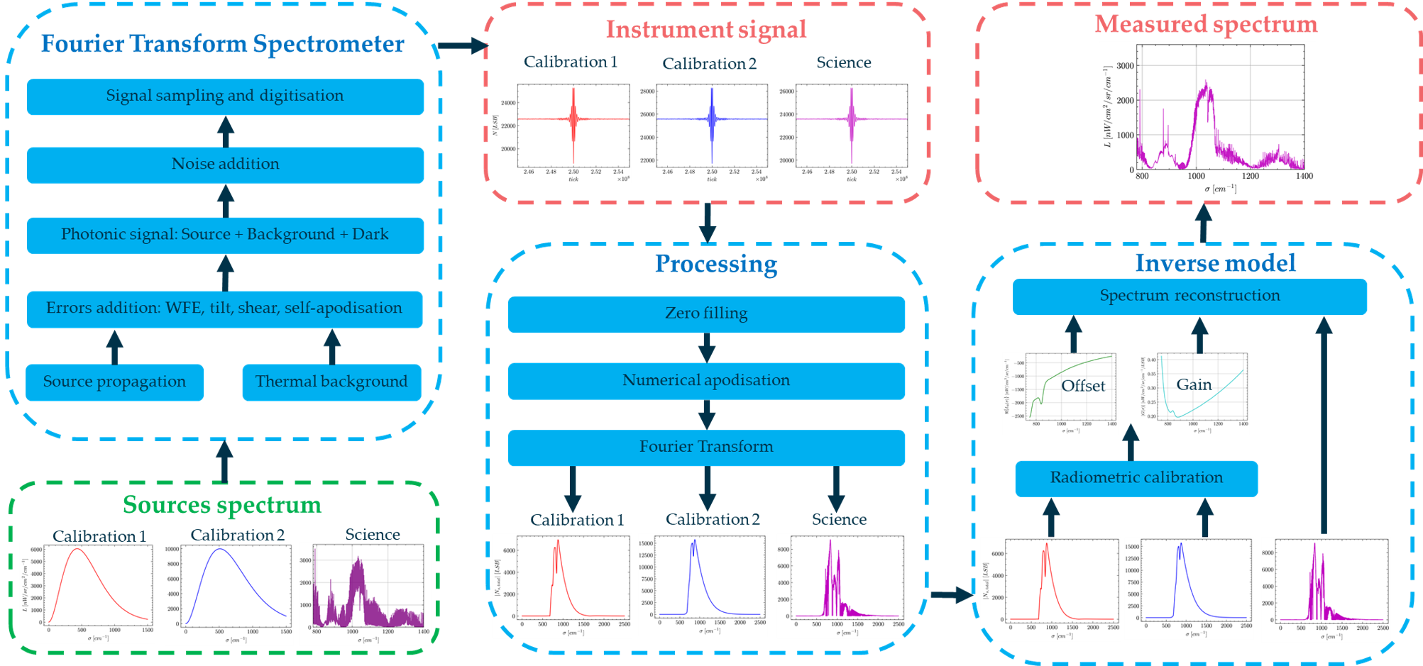
Fourier Transform Spectrometers (FTS) are cornerstone instruments in Earth observation space missions, effectively monitoring atmospheric gases in missions such as Michelson Interferometer for Passive Atmospheric Sounding (MIPAS), and Infrared Atmospheric Sounding Interferometer (IASI). It will also be the core instrument of Meteosat Third Generation – Sounding (MTG-S) and future Earth Explorer (EE) mission Far-infrared Outgoing Radiation Understanding and Monitoring (FORUM). Building on this legacy, the European Space Agency (ESA) has developed an FTS instrument and an inverse model designed to estimate the radiometric and spectral performance from a set of instrumental parameters. The model and its validation using in-flight measurements of the FTS instrument Gimballed Limb Observer for Radiance Imaging of the Atmosphere (GLORIA)-Lite are described in this paper. The results indicate that the difference between the model predictions and the measured signal is less than 2 % relative to the average of the measurements. Moreover, we can correctly predict the instrument's radiometric gain and offset and reconstruct a scientific science spectrum. This model can be utilized effectively to evaluate the radiometric performance of future FTS missions.
Keywords:
Fourier transform spectrometer
; instrument model
; radiometric performance
; radiometric calibration
; spectrum reconstruction
1. Introduction
The Fourier transform spectrometer (FTS) presents the advantage of high throughput and Signal-to-Noise Ratio compared to dispersive or filter-based spectrometers [1,2]. For these reasons, FTS have widely been used in previous Earth Observation (EO) missions to measure atmospheric trace gas concentrations. The Michelson Interferometer for Passive Atmospheric Sounding (MIPAS) developed by the European Space Agency (ESA) and launched in 2002 has observed the infrared limb emission spectrum [3]. The Infrared Atmospheric Sounding Interferometer (IASI), developed by the Centre national d'études spatiales (CNES) and operated by the European Organisation for the Exploitation of Meteorological Satellites (EUMETSAT), has measured since 2006 the atmospheric temperature and water vapor profiles, as well as greenhouse gas concentrations [4]. FTS constitute the core instrument of the meteorological EUMETSAT - ESA mission Meteosat Third Generation – Sounding (MTG-S) [5], launched on 1 July 2025, and EUMETSAT - CNES IASI – New Generation (IASI-NG) [6], which was launched on 13 August 2025 onboard MetOp-SG-A1 satellite. Several future Earth Explorer (EE) sounding and imaging ESA missions also integrate FTS as their core instrument, such as EE9 Far-infrared Outgoing Radiation Understanding and Monitoring (FORUM) [7], EE11 candidates NITROSAT [8] and Changing-Atmosphere Infrared Tomography (CAIRT) [9] for applications such as limb sounding and high spatial resolution detection of pollutants plumes.
ESA has identified the need for an FTS model for the performance prediction and design optimisation of future missions with the objective to:
- Predict the detected signal including the correct level of thermal background, dark current and noise using a set of instrumental parameters as input.
- Evaluate the instrument’s radiometric performance.
- Simulate the instrument radiometric calibration.
- Reconstruct a scientific scene spectrum.
This model is intended to be used for the optimisation of critical FTS instrumental parameters, and to estimate the impact of instrumental errors on the radiometric and spectral performance. Additionally, the model will be used to assess the effects of the radiometric calibration strategy and interferogram processing on the quality of the reconstructed scene spectral radiance.
For these reasons, in the framework of an ESA graduate traineeship [11], we have developed an instrument model capable of producing interferograms that include signal both from the source and the instrument (thermal background and detector dark current), including noise sources, at a given pixel. The model accounts for signal generation based either on a photodetector or on a pyroelectric thermal detector. Errors affecting radiometric performance such as wavefront tilt, shear, wavefront error (WFE) and integration time effects are included. The self-apodization effect is computed from the FOV geometry of the detector pixel. A key aspect of the model is the simulation of the instrument two-point radiometric calibration, with sources of reference radiances used for the reconstruction of the scientific scene spectral radiance, with associated noise propagation. We have validated the model by using real in-flight data from the FTS Gimballed Limb Observer for Radiance Imaging of the Atmosphere (GLORIA)-Lite [12]. This model was internally reviewed by ESA experts from missions such as MTG-S, FORUM, CAIRT, and NITROSAT.
This paper is structured as follows. In Section 2, we compare the model capabilities with the state-of-the art FTS models. In Section 3, we give an overview of the instrument model and present the associated assumptions. The propagation and signal conversion of both the source and thermal background flux are described in Section 4. We focus in Section 5 on the instrumental errors and effects included in the interferogram calculation. The noise model and the associated radiometric budget are presented in Section 6. We describe the inverse model in Section 7. The validation of the instrument model with in-flight measurements is presented in Section 8. The validation of the inverse model through radiometric gain and offset in-flight data is described in Section 9. Finally, a reference limb spectrum reconstruction is presented in Section 10.
2. FTS Models State-of-the-Art
We have performed a review of current state-of-the-art FTS models and compared their capabilities with the model. We extracted from this review nine models described in the literature from 1999 to 2024. Among this list, eight projects were developed by research institutes [13,14,15,17,18,19,20,21] and one by industry [16]. This selection includes models developed in European [16,20,21], American [13,14,19], Canadian [16,17] and Chinese [15,18] organisations.
The criteria used for the first part of this comparative study and listed in Table 1 are the following:
- Design flexibility: the model is suited to study different instrumental designs and is not adapted to only one specific design. The optics architecture, performance and temperature in the instrument can be modified without a source code update.
- Photodetector: the model can provide signals assuming a photodetector and relying on a flux-to-signal conversion model [26].
- Thermal detector: the model can provide signals assuming a thermal detector and relying on a flux-to-signal conversion model [26].
- Interferogram simulation: the model can generate an interferogram sampled on an analog or digitized axis.
- Radiometric calibration: the model implements the observation of calibration sources, calculating calibration interferograms used to estimate the instrument gain and offset [27].
- Spectrum reconstruction: The science scene spectrum is obtained from the science interferogram and the instrument radiometric gain and offset [27].
A model, developed at the Rochester Institute of Technology, uses the Digital Imaging and Remote Sensing Image Generation (DIRSIG) [13] to generate and propagate a temporal varying scene in the instrument to create an interferogram from a photodetector model only. The spectrum is reconstructed only by a Fourier transform of the associated interferogram. No radiometric calibration using reference sources is simulated. The same capabilities were found in a model developed at the same institute [14] which targets airborne detection of fugitive gases, and in a simulator from the Chinese Academy of Sciences and the Hefei University of Technology [15] which is based on the spectrometer HJ1A-HSI that monitors Earth land and vegetation.
Based on MIPAS heritage, a simulator for IASI has been developed by ABB which manufactured the mission interferometer [16]. It simulates an interferogram to predict IASI future performance and provide test data for the development of processing algorithms. However, the description of this simulator is limited to the interferogram realisation without any spectrum reconstruction. A generic model of FTS spectral response, built in the frame of a doctoral thesis at Université Laval, is described in [17] but does not study the radiometric aspect of the instrument by modelling the optics or detector efficiencies. A Michelson interferometer simulator that was developed by the China Meteorological Administration, the Chinese Academy of Meteorological Sciences and the Beijing University of Technology, based on the Geostationary Interferometric Infrared Imager (GIIRS) is presented in [18] to specifically study the effects of the pixel response non-linearity and off-axis angle on the spectrum. This model does not have the capabilities to estimate the instrument’s radiometric performance, and the radiometric calibration is not simulated to compute the scene spectral radiance.
A numerical tool developed at the James Madison University, called Fourier Transform InfraRed Scientific Instrument Simulator (FTIR-SIS) is presented in [19]. It can generate a scene from a selection of atmospheric molecules, simulate two different predefined materials for the gas cell window, the beam splitter plates, and the detector window. One can also choose between two predefined photoconductor or thermal detector responses. However, only the spectral flux incident on the detector is visible. No interferogram is simulated and no science spectral radiance is reconstructed. The instrument radiometric performance cannot be estimated from FTIR-SIS. An E2E instrument simulator of the concept of Far Infra-Red Interferometer (FIRI) has been developed at the University College London and Leiden Observatory [20]. It specifically targets the observation of sub-arcsecond astronomical objects such as circumstellar disks. The scene reconstruction is performed using the CLEAN algorithm which is a method developed for radio astronomy. No radiometric calibration is simulated. Finally, a Simulator for the Herschel Imaging Fourier Transform Spectrometer (SHIFTS) model has been developed at the University of Lethbridge the and the Rutherford Appleton Laboratory, based on the Spectral and Photometric Imaging Receiver (SPIRE) which observed in the FIR and millimetre band [21]. Only SPIRE bolometer detection technology is modelled, and as [20], no radiometric calibration is simulated.
We now focus the comparative analysis on criteria relative to the instrumental effects, error and noise listed in Table 2 and defined as follows:
- Instrument thermal background: the thermal self-emission of the instrument is considered to calculate the output signal and/or the noise levels.
- Interferometer modulation losses: the wavefront error (WFE), tilt and shear between the wavefront recombined in the interferometer are considered to calculate the performance [28].
- Self-apodisation: the Self-apodisation induced by the optical path difference in-field variation is considered to assess the performance and to calculate the output signal [30].
- Detector non-linearity: the non-linearity of the detector response is considered to calculate the output signal [29].
- PRNU: the pixel response non uniformity (PRNU) [31] is considered to calculate the output signal.
- Integration time effect: the impact of integration time on the interferogram contrast effect due to flux temporal integration is considered to calculate the output signal and the radiometric performance [32].
- LOS jitter error: jitter due to fluctuation of the line of sight (LOS) during the observation of an inhomogeneous scene is considered to estimate the output signal and the radiometric performance [33].
- Sampling error: the non-regular sampling induced by the dynamic mirror displacement velocity variations is considered to calculate the output signal and the radiometric performance [34].
The instrument thermal background, critical in the IR range, is only considered in the IASI [16], FIRI [20] and SPIRE [21] simulation models, as the first one targets long wave infrared scene and the two other are sensitive to the FIR. The other models do not include this contribution either because 1) they primarily focus on the impact of effects such as PRNU, sampling errors and LOS jitter errors [13,18], 2) they study a spectral band where this contribution is negligible [21], or 3) they are not developed to estimate the instrument radiometric performance [17,18,19] which is why they do not consider the detector noise. The interferometer modulation losses resulting from imperfect surfaces and alignments in the interferometer which reduce the integrated spectral flux [28] are taken in account in [16,17]. The effect of the temporal integration of the flux during the signal acquisition, is modelled in [15,16]. The effect of the detector response non-linearity is only included in [16] and [18].
Based on the listed model capabilities, we estimate that [16], [20] and [21] can be used for the evaluation of an FTS radiometric performance as they both consider the instrument thermal background and the detector noise. However, [20] and [21] are designed for specific astronomical applications in the FIR and mm range. They do not consider errors such as shear, tilt and WFE which impact radiometric performance. IASI simulator [16] includes these effects and appears to be the most flexible model for a radiometric budget evaluation. However, the description of this model stops at the generation of the interferogram. No reconstruction of a scene spectral radiance is presented. The instrument’s spectral performance, impacted by self-apodisation, is thus not visible on the spectrum. Spectral performance can be evaluated with [17] which focuses on this aspect and consider radiometric performance out of its scope. In general the effect of self-apodisation on the spectrum is studied in [16,17,18].
One key aspect of this study is also the validation of these models. Among the nine communications we cited, three mentioned a validation. IASI simulation model validation is based on the heritage of an FTS simulator developed for MIPAS at ABB Bomem [16], but no related communication is available in the literature. SHIFTS model results have been compared with real HERSHEL-SPIRE measured spectra [21]. This comparison showed a correspondence between simulated and real data of SPIRE second band (31 cm-1-55 cm-1), but there is an important difference in the first band (14 cm-1-34 cm-1) where “synthetic” (modelled) spectra contain up to five times more energy than observed real data. A comparison between the spectral response model described in [17] and real instrument line shape (ILS) measurements validated this model. But as previously mentioned, only the spectral performance of the instrument is studied.
We notice that state of the art models designed to be flexible [13,14,16] either do not simulate the instrument radiometric calibration and spectrum reconstruction [16], or do not consider key effects as thermal background [13,14]. This last point prevents us from evaluating the radiometric performance in and near the IR range. Some other reviewed models include errors we do not consider in the model as the LOS jitter and the sampling errors [20,21]. We did not include these effects as, in our applications, they were minor contributors to the radiometric performance budget compared to noise and error contributions detailed in Section 5 and Section 6. These models [20,21] were developed to assess the performance of a specific instrument design and application as millimetric astronomy. Finally, only limited communication is made about the validation of these models.
We have combined six major innovations and novelties in the model developed at ESA. First, the model is flexible and can be adapted to a wide range of instrument designs. Second, this model provides the capability to either use a photodetector or a thermal detector and is thus suitable for a large spectral domain from ultraviolet (UV) to FIR. Third, it uniquely combines the reconstruction of a scene spectrum based on the instrument's radiometric calibration with the realistic simulation of noisy interferograms from three different sources. The instrument and inverse models, along with their associated code, can be run independently or collectively to simulate three interferogram acquisitions and reconstruct the science spectrum with a single execution. The quick execution time of both the instrument and inverse model codes, which is less than 10 seconds in our environment, enables a rapid evaluation of the impact of instrument design parameters on performance. This facilitates the use of the model to an perform error analysis as we proceed in Section 8, and further to evaluate the instrument absolute radiometric accuracy [35]. Finally, this model predicts the level of the signal’s minimum, maximum and average levels with an accuracy better than 2 %, as shown in Section 8.
3. Instrument Model
3.1. Instrument Model Overview and Assumptions
Figure 1 represents the instrument model block diagram. The input is a spectral radiance from either a scientific source provided by an atmospheric radiative transfer code, or a known calibration source such as a blackbody. The instrument model comprises the following sub-systems: The scan mirror, the front telescope (FT), the interferometer assembly (IA), the back telescope (BT), the spectral filter, the cryostat window (CW), the detection unit (DU) and the analog-to-digital converter (ADC). The flux at the instrument output is converted into a signal by the DU which also adds the dark signal (in case of a photodetector) and the noise. The signal provided by the DU is digitized by the ADC that provides as outputs the scientific and calibration signals.
The model can simulate a filter positioned either in the cryostat (Figure 2) or between the BT and the CW. The input beam is incident on the scan mirror that reflects the beam toward the FT and the IA that comprises a beam-splitting unit (BSU), and two cube corners CC1 (static) and CC2 (dynamic). The BSU reflects a fraction of the incident beam towards CC1 and transmits the other fraction toward CC2. During the data acquisition, CC2 is translated at the optical speed vopt defining the optical path difference (OPD) scanning rate. For a duration Δt, the associated scanned OPD range is thus vopt×Δt. The beams reflected by CC1 and CC2 are incident on the BSU and transmitted and reflected toward the BT respectively. The recombined beams transmitted by the BT are focused on the DU and pass by the CW, the spectral filter. The intermediate pupil ΦI is located at the CC1 apex and the entrance pupil ΦE is located at the scan mirror vicinity. The aperture stop is located at the detector box entrance and reimaged on the cube-corner apex. The detector is the system field stop.
We consider a step-and-stare observation method [36], with the barycentre of each pixel projected on the scene being static during the signal acquisition. The aberrations of the pupil imaging are considered negligible. Each optical sub-system is aplanatic, with a transmission Κ and an operating temperature T. The optical etendue is conserved through the instrument [37]. We neglect the contribution to the measured flux of the spurious reflections on the interferometer BSU plates, the CW, the filter, and the detector faces. The BSU comprises a beam splitting surface (BS), a beam splitting plate (BP), and a compensation plate (CP). The BP is coated with anti-reflective (AR) coating on one side and BS coating on the other, while the CP is AR coated on both faces.
We assume that an ideal metrology correction is applied on the interferogram such that 1) the CC displacement is linear, 2) the interferograms are regularly sampled and centred on the zero-path difference (ZPD). The detector is assumed to be photoconductive or pyroelectric. The photodetector noise budget comprises the following contributors: source, instrument thermal background and dark current shot noises, readout noise, ADC digitisation noise, Johnson [26] and KTC [38] noises. The pyroelectric detection unit noise budget comprises the ADC digitisation noise, the detector noise, the amplifier noise. The detector and amplifier noise can be provided by the manufacturer. In this case, the “detector noise” mainly includes the thermal fluctuation noise and the Johnson noise and is thus rather independent from the source [40].
3.2. Beam Splitting Unit Model
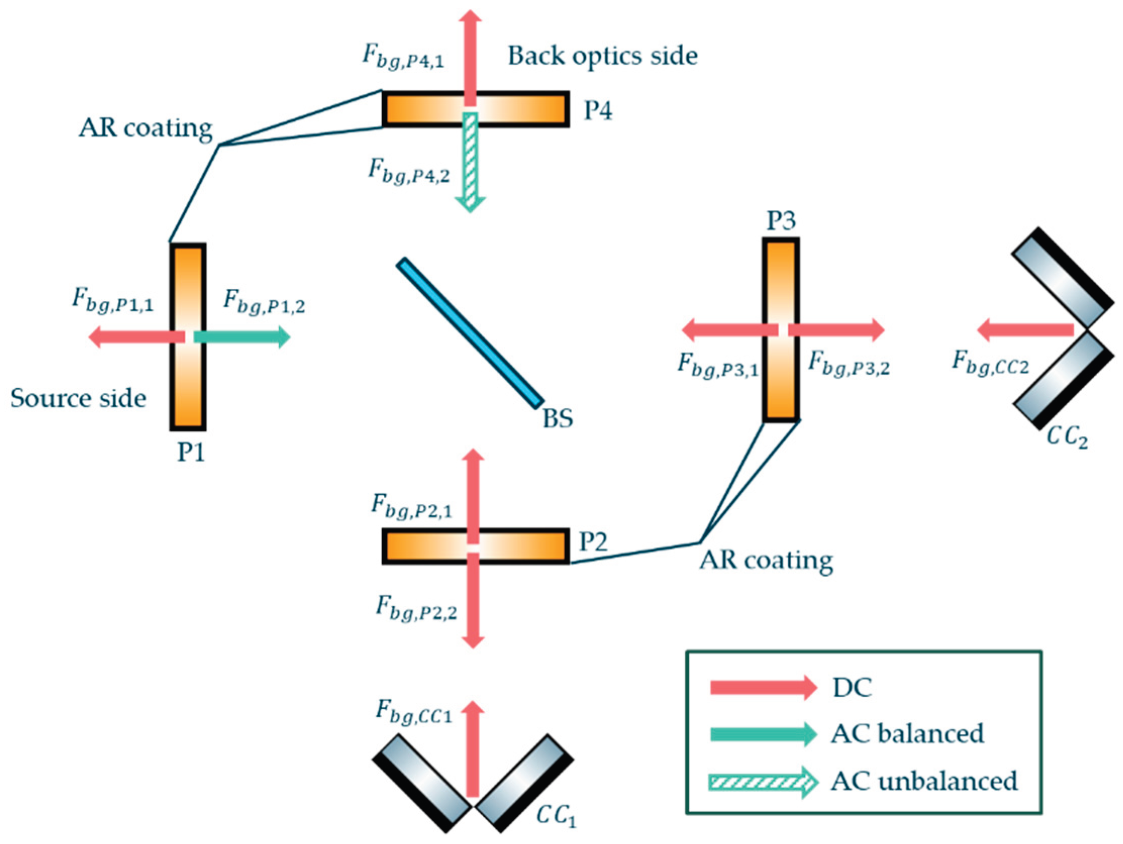
The BSU model is represented in Figure 3 and allows simulating various BSU architectures [41]. A perfect, non-absorbing, zero-thickness BS plate is positioned at the centre. The BP and CP are divided into two plates called P1 and P2 (for BP) and P3 and P4 (for CP). It is important to notice that P1 and P2 (for BP) and P3 and P4 (for CP) have the same thickness (hBP for BP and hCP for CP), orientation, and material characteristics as BP and CP, respectively. We disregard any spurious reflections on their surfaces.
The absorption of each plate α is determined by the material absorption rate β per unit of optical thickness h:
where σ is the wavenumber. The crossed thickness of each plate depends on the mechanical thickness d, the beam incidence angle ϕ, and the material optical index n:
3.2. Detector Model
3.2.1. Photodetector Signal
For a spectral flux incident on a detector F, the photodetector flux-to-signal conversion is characterized by the pixel fill-factor ρ, the integration time τint, the detector quantum efficiency (QE) η, and the energy of a photon hcσ. The unmodulated (DC) signal NDC associated to an unmodulated spectral flux FDC is expressed as follows:
The modulated (AC) signal NAC associated to a modulated spectral flux FAC is expressed as follows:
where δ is the OPD and R{FT} denotes the real part of the Fourier transform. The quantities O and M are the instrument function and modulation efficiency which are described later in Section 5. This approach is valid both for the incident source and background flux. The total photonic signal Nph is the sum of the modulated and unmodulated source Ns, background Nbg and dark signals Ndark (Figure 4 left panel):
3.2.2. Pyroelectric Detector Signal
A pyroelectric detector is only sensitive to the modulated signal [26]. The flux-to-signal conversion is modelled using the detector voltage response RV and material absorbance αpyr. The voltage response depends on the electric frequency fel which, for an FTS has a direct relation with the wavenumber σ. Using the optical speed vopt, we can write σ= fel / vopt (equation 2.11 in [42]) and express the pyroelectric signal equation with the wavenumber:
The total signal converted by the pyroelectric detector Npyr is the sum of the modulated source and background signals.
3.2.3. Signal Digitisation and Sampling
The signal is sampled according to the detector’s acquisition framerate facq and the optical speed such that the OPD sample size equals vopt/facq. The ADC digitizes the signal according to its effective number of bits (ENOB), the charge handling capacity (CHC) in the specific case of a photodetector, and the maximum voltage swing for a pyroelectric detector. Figure 4 right panel shows the sampled digitized signal in least significant bits (LSB) obtained from the total photonic signal in mega electrons of the left panel.
3.2.4. Non-Linearity
The detector response NL is defined as the relative difference between the signal that would be provided by a detector with an ideal linear response NE and the actual detected signal N [43,44]:
where the NL function is modelled as a 3rd order polynomial characterized by the coefficients {a0; a1; a2; a3}:
For a detector with an ideal linear response, the coefficient a0 equals one and the others equal zero.
3.2.5. Noise Budget
The noise budget for the photodetector model includes the standard deviation of 1) the source shot noise ξshot,s, 2) the background shot noise ξshot,bg, 3) the dark shot noise ξdark, 4) the readout noise ξread, 5) the Johnson noise ξJohn, 6) the KTC noise ξKTC and 7) the ADC digitisation noise ξADC. These noises are considered independent such that the total noise variance ξ2 is the quadratic sum of all its contributors. We also include in the noise budget the factors of pixel spatial binning bspat and acquisitions temporal averaging btemp. The expression of the standard deviation of the total noise detected by the photodetector DU is thus:
The contributors to the pyroelectric DU model noise budget include the standard deviation of the detector noise ξdet, the amplifier/filter chain noise ξamp and the ADC digitisation noise. In this case, the expression of the standard deviation of the total noise is thus:
4. Flux Incident on the Detector
4.1. Source Flux
The source spectral radiance Ls is converted into an entrance spectral flux FE using the instrument optical etendue G.
The source spectral flux incident on the detector Fs is:
where Fs,DC the unmodulated flux and Fs,AC the modulated flux can be expressed using FE and the DC and AC optical transmissions of the instrument (ΚDC, ΚAC):
ΚDC and ΚAC are the products of each sub-system optical transmission Kj with j = {scan, FT, IA, BT, CW, filter}:
ΚDC and ΚAC differ in the IA unmodulated and modulated optical transmission (ΚIA,DC and ΚIA,AC), respectively, which depend on the CC reflectivity RCC, the BS transmission and reflectivity (ΚBS,RBS), the plates absorption coefficient αP and the AR coating transmission ΚAR. For the sake of clarity, we will omit the spectral dependency symbol "(σ)" in Section 4 for each transmission and reflectivity factor, only including it at the end. The expression of ΚIA,DC and ΚIA,AC are:
The IA reflects the back optics self-emitted flux as explained in the next section 4.2. with the following reflectivity factors RIA,DC and RIA,AC:
4.2. Thermal Background Flux
4.2.1. Unmodulated Thermal Background Flux
All the instrument sub-systems emit a DC self-emission flux directly emitted toward the detector (red arrows in Figure 5) that contribute to the background flux. Their individual expressions Fbg,j,DC with j = {scan, FT, IA, BT, CW, filter} are:
where LBB is the Planck’s law radiation [42], ε the emissivity, T the temperature and ADU the studied active detection area.
Because the filter is located inside, its self-emission is integrated over the full projected half space π [45]. Each sub-system's emissivity is calculated as one minus its transmission and reflectivity, except for the IA, which is detailed in Appendix A.
4.2.2. Balanced Modulated Thermal Background Flux
The flux emitted by a component located between the entrance pupil and the IA is modulated in phase with the source flux ('balanced output' in [46]). As represented by green full arrows in Figure 5, the scan mirror, the FT and the IA BP (see Figure 17 in Appendix A) emit a balanced background flux (Fbg,scan,AC, Fbg,FT,AC, Fbg,IA,AC,1) expressed as:
4.2.3. Unbalanced Modulated Thermal Background Flux
The flux emitted by a component located between the IA and the DU is reflected by the interferometer towards the detector. It is modulated in phase opposition with the source flux ('unbalanced output' in [46]). As represented by green dashed arrows in Figure 5, the IA CP, the BT, the CW and the filter (see Figure 17 in Appendix A) yield the following unbalanced modulated background flux incident on the detector (Fbg,IA,AC,2, Fbg,BT,AC, Fbg,CW,AC, Fbg,filter,AC):
where the minus sign in equation characterizes the unbalanced modulation.
4.2.4. Detection Unit Thermal Background Flux
The detector cryostat thermal is integrated over the full half space π, minus the source beam solid angle. The cryostat emissivity is assumed to be equal to 1 and the associated unmodulated background flux Fbg,DU,box
is:
A fraction of the detector's self-emission beam travels through the filter, the CW and the BT towards the IA, where it is reflected back towards the detector. The flux incident on the detector following this optical path is:
where absorption αDU,mat is the detector material absorbance.
In the case of a photodetector located in a cryostat the term Fbg,DU,mat is neglected. In the case of a pyroelectric detector insensitive to unmodulated signal, Fbg,DU,box is not considered.
5. Instrumental Degradations and Spectral Response
5.1. Modulation Efficiency
The instrument is subject to errors associated with the quality of optics and misalignments which consequently diminishes the interferogram contrast [28]. We assess the associated contrast by using the modulation efficiency M.
where Mtilt is the contrast loss associated to the angular tilt between the two interfering wavefronts, Mshear represents the contrast loss due to the shear between these wavefronts, MWFE is the contrast loss induced by the differential WFE between the two interfering waves and Mτint is associated to the signal integrated over the exposure time τint. In the model, the instrument errors are assumed to be static during the acquisition.
Mtilt associated with the angular tilt between the two interfering wavefronts γtilt, an aperture stop of equivalent radius Rstop writes, using the Bessel function of first kind J1, as follows [28]:
Mshear corresponding to the contrast loss induced by the shear γshear and a solid angle Ω writes as follows [47]:
The contrast loss induced by the differential WFE between the two interfering waves MWFE induced by the differential WFE between the two interfering wavesΔδ2 is [28]:
The contrast loss Mint associated to the signal integrated over the exposure time τint. during the dynamic CC motion at constant optical speed vopt is expressed as [32]:
5.2. Self-Apodisation and Spectral Response
Self-apodisation is due to the OPD in-field variations [30]. The output flux F of an off-axis beam propagating inside the IA with an off-axis angle θ0 is [30]:
The flux incident on the detector for a beam propagating in the angular direction angle θ0 and of solid angle Ω is [30]:
where, cosθ0(1-Ω/4π) is equivalent to a shift of the wavenumber, and Oapo is the term representing the self-apodisation instrument function component acting on the interferogram contrast [28].
It is important to mention that Oapo depends both on the wavenumber and the OPD and that the impact of the self-apodisation on the contrast is maximum at σmax. In the model, we therefore decided to compute the instrument function at σmax.
The other contributor to the instrument function is the restriction on the OPD range due to the restricted displacement range of the dynamic CC. The signal is acquired between -MOPD and +MOPD where MOPD is the maximum optical path difference. The associated contributor Orange to the instrument function is represented as a unit boxcar function [30]:
The global instrument function is:
The spectral response, named instrument line shape (ILS) is defined as the real Fourier transform of the instrument function.
The resolution-limited spectrum measured by the instrument is therefore the convolution of the entrance spectrum with the ILS. In this paper, the spectral resolution is defined as the ILS central lobe full width at half maximum (FWHM). Figure 6 represents the focal plane (left panel) and the ILS (right panel) of the GLORIA instrument at σ = 1400 cm-1, an MOPD of 8 cm, an FOV of 26.6 × 70.9 mrad2 and a pixel FOV of 0.56x0.56 mrad2 [12]. On the right panel, we estimate that the on-axis ILS FHWM is equal to 0.0753 cm-1 while its FWHM increases to 0.0764 cm-1 for the beam propagating at the top left corner pixel of angular coordinate (13.3 mrad; 35.4 mrad). In this figure, we notice that the relative spectral shift of the wavenumber cosθ0(1-Ω/4π) equals 0.9993 which displaces the line at σ = 1400 cm-1 to σ = 1399.016 cm-1.
6. Radiometric Performance Budget
In this section we calculate two common metrics to estimate the radiometric performance : the Noise Equivalent Spectral Radiance (NESR) and the Noise Equivalent Differential Temperature (NEDT)
7. Inverse Model
7.1. Inverse Model Overview
The inverse model (Figure 7) retrieves a spectrum from two input calibrations and one input science interferograms provided by the instrument model. The outputs of the inverse model are the scene spectral radiance, the instrument radiometric gain and the radiometric offset including their respective noises. The reconstruction process comprises three steps described hereafter. First, we estimate the radiometric gain and offset from the Fourier transform of the two calibration interferograms using a two-points method [27] as described in section 7.2. Second, we reconstruct the scene spectrum from the Fourier transform of the science interferogram by using the radiometric gain and offset. Finally, the model propagates the noise in the reconstruction process as detailed later in section 7.3.
7.2. Radiometric Calibration and Spectrum Reconstruction
The instrument model provides a modulated signal NAC. We include the possibility to perform zero-filling on the signal to interpolate the spectrum and accelerate the Fast Fourier Transform algorithm as well as performing a numerical apodisation to mitigate the “ringing” phenomenon [42]. The complex signal in the spectrum domain Nσ is the Fourier transform of the modulated signal.
The relation between Nσ, the entrance spectral radiance L, the instrument complex radiometric gain G and offset L0 is [27]:
The gain and the offset are estimated from the acquisition of two calibration sources (1,2) with known spectral radiances (L1,L2) associated with two complex signals (Nσ,1,Nσ,2):
and:
The spectral variability of G is induced by the optical transmission of the instrument, the response of the detector, and the modulation loss. The offset radiance L0 is caused by the modulated self-emission of the instrument.
7.3. Noise Propagation in Spectrum Reconstruction
In addition to a numerical propagation of the interferogram noise to the spectrum, we also analytically assess this propagation in the reconstruction equations. To estimate the spectrum noise standard deviation ξL, we start from inserting equations (52) and (53) into (51) to get an explicit expression of the reconstructed spectral radiance Ls as function of the calibration and scene signals:
The noise between distinct signal acquisitions is assumed to be uncorrelated and the propagation of both the calibration and scene signal noise can be expressed accordingly.
Thus yielding:
We deduce that:
This last formulation highlights the relation between the instrument's radiometric performance (NESR), the dynamics between the different calibration and scientific source spectral radiances and the reconstructed spectrum noise standard deviation. Equation (58) can also be written in terms of noise temperature using equation (49). It is important to notice that the numerical apodisation of the interferogram is not included in this consideration.
This method enables an evaluation of both the instrument's radiometric performance and the calibration strategy regarding their effects on the quality of the reconstructed scene's spectral radiance. It is important to notice this section exclusively details the analysis of the reconstructed spectrum noise propagation while the model also evaluates the noise on the gain and the offset (see Appendix B).
8. Instrument Model Validation
8.1. The GLORIA-Lite Instrument
GLORIA-Lite (Figure 8) is an atmospheric limb emission sounder built and operated by the Karlsruher Institut für Technologie (KIT) and the Forschungszentrum Jülich (FZJ). It has crossed the Atlantic on a stratospheric balloon in June 2024 and delivered several terabytes of limb emission spectra during this mission [52].
GLORIA-Lite is a double pendulum interferometer with fixed plane retroreflectors. The interferometer uses a diamond beamsplitter without any compensation plate. The moving mirrors are two CCs mounted on a rotating structure and provide an MOPD of 25 mm. The back optics is a fully reflective design with an effective focal length of 60 mm. The operation temperature is ambient, which means that the instrument drifts thermally in the range from 20 °C to –20 °C during the balloon flight. The detector system is a mercury cadmium telluride (MCT) large focal plane array (LFPA) with 15 µm pitch operating at 75 K and covers the thermal infrared spectral region. A 2 × 2 hardware binning and a 1 × 48 software binning are used to achieve a spatial sampling of 300 m × 14 km at the horizon. Two calibration sources, a blackbody, that is radiatively cooled, and deep space are used for determination of radiometric offset and gain.

Table 3.
GLORIA-Lite essential properties.
| Property | Value |
| Mass | 35 kg |
| Power consumption | 80 W |
| Spatial sampling at horizon | 300 m × 14 km |
| Spectral sampling | 0.2 cm-1 |
| Spectral coverage | 750 - 1390 cm-1 |
| Sensitivity | ~10 nW/(cm² sr cm-1) |
8.2. Validation with GLORIA-Lite in-Flight Signals
In this section, we present an analysis of GLORIA-Lite signal measurements consisting of Level-0 processed in-flight data [53] that we compare to the model predictions. This, while observing a 241.316 K blackbody and the deep space. It is important to mention that GLORIA-Lite is a balloon borne embedded instrument located at an altitude where the so-called “deep space source” is not very “deep”, and some atmospheric residuals are included into these measurements [54]. KIT has measured and provided this additional emission such that in the model, the spectral radiance of the deep space source corresponds to the one measured by GLORIA. We implemented GLORIA-Lite layout into the model by inputting the instrumental parameters provided by KIT and described in 8.1.
For each GLORIA-Lite detector pixel, the in-flight DC level is computed as the average of the first and last 2000 frames signal, which corresponds to an OPD range of 0.4 cm as represented on Figure 9. We noticed that the difference in the DC levels between the first and last frame calculation is negligible (<0.1 %), and we thus decided to show the figures related to the first 2000 frames only.
On the deep space acquisition, the model predicts 7.07 Me- for baseline and 7.86 Me- for ZPD levels, with atmospheric residuals and dark current accounting for about 0.6 % and 5 % of the total DC photonic level, respectively (Figure 10). The instrument self-emission represents here more than 94 % of the total signal thus constituting the major contributor.
We represent on Figure 11 left panel the signal of a deep space acquisition obtained by the model (red) and measured during GLORIA-Lite flight (blue), at the central pixel. Figure 11 middle and right panels respectively show the histograms of DC and ZPD signal measurements over the whole detector, versus the level predicted by the model (red dashed line). The measured baseline and ZPD levels are 7.15+/-0.16 Me- and 7.86+/-0.16 Me-, respectively. The model predictions thus lie in the range of these measurements. The standard deviation of the signal histogram represents between 2 % and 2.5 % of the average signal that corresponds to a typical level of detector PRNU [55]. The agreement between predicted and measured average signals validates the ability of the model to predict the signal dynamic of a “Deep sky source”.
We performed the same analysis on the signal acquisition of a 241.316 K blackbody (Figure 12). Looking at the DC and ZPD signals over the detector (middle and right panels), the measured baseline and ZPD level are 8.50+/-0.16 Me- and 7.11+/-0.15 Me-, respectively. The model predicts a baseline level of 8.61 Me- and a ZPD level of 7.14 Me-. As for the deep space view, the model predictions are in good agreement with the measurements. This validates the model capability to predict the signal dynamic of a blackbody calibration source.
We conclude that the model can successfully predict the DC and ZPD signal levels of two calibration sources: deep space, including atmospheric residuals and a 241.316 K blackbody. The maximum observed relative difference between the prediction and the average signal measurements dN is only 1.3 % on the blackbody baseline level, with dN defined as:
where Nmodel and Nmeas are the predicted and measured signal, respectively. We attribute these differences to:
- The error on the temperature of the elements located between the scan mirror to the CW which is estimated to be equal to 0.5 K.
- The error on the dark current density associated with the in-flight detector measured temperature uncertainty of 0.03 K . The consequent dark current drift is deduced from the “Rule07” associated to MCT infrared photodetectors [56] and is equal to 2.16 mA/m2.
- The detector PRNU which we assume equal to 2%.
- The error on the blackbody emissivity which is estimated to be equal to 0.003 based on GLORIA calibration source stability requirement [57].
- The error on the blackbody temperature which is estimated to be equal to 0.03 K based on in-flight temperature measurements precision.
- The error on the mirrors coating reflectivity which is estimated to be equal to 0.0005. There is one mirror in the front optics, seven per CC assembly and four in the back optics.
- The error on the BS substrate transmission which is estimated to be equal to 0.005.
- The error on the BP thickness which is estimated to be equal to 0.05 mm.
- The error on the BP AR coating reflectivity which is estimated to be equal to 0.0005.
We performed an error analysis on this set of uncertainties to estimate their influence on the error of the blackbody signal estimation. We assume the listed errors to be uncorrelated. The total signal error ΔN is the quadratic sum of each contributor ΔNi related to a parameter ui:
where Δui is the uncertainty or error associated with a signal error ΔNi.
Table 4 presents the estimated error budget. The largest contributors of the baseline error ΔNDC are the PRNU, the optics temperature and the mirrors reflectivity that contribute to 1.95 %, 0.67 %and 0.64 % of the error made on the DC signal, respectively. Furthermore, the instrument thermal background dominates the radiometric budget as it represents about 68 % of the total DC signal. It is thus expected that minor changes in the transmission of optics and temperature have a significant influence on the predicted signal measurements. The errors on the blackbody emissivity, the IA plate AR coating reflectivity and the plate size, contributing to 0.17 %, 0.16 % and 0.14 %, respectively, are of secondary order compared to the first three contributors. The contributions of the BS transmission, the dark current and the blackbody temperature are considered as fully negligible. The total error represents 2.16 % (0.19 Me-) and 2.37 % (0.17 Me-) of the model baseline and ZPD signals, respectively. These results are in good agreement with the standard deviation of the measured signal distribution.
9. Radiometric Calibration Model Validation
In this section, we validate the radiometric calibration model by comparing radiometric gain and offset predictions and measurements. Contrary to the acquisitions presented in Section 8, signals are here normalized to a similar integration time of 100 μs. Atmospheric residuals of the deep space signal are already corrected in GLORIA-Lite measurements as part of the L1 data processing [54]. For this comparison, we thus did not include these residuals in the simulated deep space acquisition.
Figure 13 represents the instrument radiometric absolute gain (left panel) and offset real part (right panel) predicted by the model, compared to the measurements between 780 cm-1 and 1400 cm-1. Gain is low in this range where GLORIA-Lite optics transmission and detector response are optimized. The offset is negative because most of the instrument thermal self-emission comes from the back optics and the CW.
We see a good agreement between the predictions and the measurements which shows a good knowledge of optics and detector response, as well as the instrument temperatures. For the gain, the biggest difference between the model predictions and the measurements is located between 800 cm-1 and 1000 cm-1 where measurements values are between 10% and 25% higher. We attribute this to an overestimation of the material and AR coating transmission from the CW and the IA plate. The input transmission curves for these two components are based on their material bulk absorption and thickness but not on independent measurements performed on the instrument.
We also notice fluctuations between 800 cm-1 and 1300 cm-1 with an approximate period of 100 cm-1. We attribute these fluctuations to the Fabry-Perot channelling effect occurring in the detector substrate [58,59]. Let ‘s assume this substrate has a thickness d and a refractive index n. The optical path difference between a nominal beam normal to a surface which is directly transmitted and a secondary beam that is reflected twice before equals 2nd. This corresponds in the spectrum domain to a beating frequency of Δσ=1/2nd. We assume that the HgCdTe detector substrate has a refractive index of approximately 3.3 [60]. For such detector optimized for very long wave infrared (VLWIR), we estimate that the substrate thickness is equal to 15 µm [56]. This results in Δσ≈100 cm-1 which agrees with the observed gain oscillations frequency as represented in Figure 13 left panel. The other refractive surfaces as the IA plate and the CW are wedged to avoid this effect.
Looking at the offset, we predict up to 20 % lower L0 absolute values compared to measurements between 800 cm-1 and 850 cm-1, likely because of the underestimation of the CW transmission. This is in accordance with the higher gain measurements in this region. The fluctuations in offset measurements between 950 cm-1 and 1300 cm-1 agree with fluctuations observed in the gain in this range. In this region, we slightly overestimate L0 probably due to the underestimation of the IA plate transmission. Such fluctuations in optics transmission are usually not considered in feasibility studies where manufacturing and testing have not started yet. We thus conclude that the model can predict the instrument’s radiometric response and offset.
10. Inverse Model Validation
In this last section, we use both the instrument and inverse models to reconstruct a spectrum in the GLORIA-Lite spectral range. The reference scene is a 20 km altitude, mid latitude day limb reference spectrum [61]. For the radiometric calibration, we simulated the averaging of 10 acquisitions of both deep space and blackbody. We also coadded the 48 pixels in the horizontal direction to mitigate noise as performed on the previous balloon-born version of GLORIA [62].
The “original” spectrum has a 0.05 cm-1 spectral resolution while the instrumental resolution is 0.385 cm-1 after application of a Norton-Beer strong apodisation [63]. An illustration of the reconstruction is presented in Figure 14. Spectrum across the full spectral range is represented at the top left panel while zoomed views over 10 cm-1 ranges are displayed on the other panels.
In the bottom right panel, we notice that the model can reconstruct emissions lines characteristics of Sulphur Hexafluoride (SF6) around 950 cm-1. The top right panel includes a retrieval region of Ozone (O3), while the bottom right panel represents a retrieval region of the Sulphur Dioxide (SO2). The observation of these three atmospheric gases is targeted by the EE11 CAIRT candidate [9].
In a second time, we compare the model reconstructed spectrum with a theoretical spectrum corresponding to the instrument’s apodized spectral resolution. As represented on Figure 15, this theoretical spectrum is the convolution of the “original” spectrum with the ILS considering a Norton-Beer strong apodisation. On Figure 16, this spectrum is compared with the noiseless spectral radiance from the model, examining the same three spectral ranges as presented in Figure 14. We observe that both the theoretical (red dashed lines) and the inverse model (green lines) spectral lines match. This agreement confirms the capability of the model to simulate the retrieval of a scientific source spectrum considering the instrument’s spectral response and radiometric calibration.
11. Conclusion and Discussion
We have developed at ESA an FTS radiometric model to support future EO missions in phase 0/A. It is divided into an instrument and an inverse model we both described in this paper. Based on a versatile beam splitting unit model and two different types of detectors, the instrument model simulates noisy digitized interferograms both from input calibration and scientific sources. The retrieval model simulates the instrument radiometric calibration, reconstructs the scene spectral radiance and propagates the signals noise in the process.
The ESA model and the corresponding code are designed to be adaptable to various instrumental parameters. This allowed us to simulate the design of various mission payloads such as CAIRT, NITROSAT, GLORIA-B and GLORIA-Lite which has been used for the model validation. The comparison between the model signal predictions and actual in-flight measurements indicated a maximum deviation of less than 2% for both the baseline and ZPD levels relative to the average measured levels. We are also able to predict with a good precision the instrument radiometric gain and offset, considering the uncertainties on the instrument parameters. This validates the capability of the model to accurately estimate the instrument’s radiometric performance in phase 0/A. A reconstruction of a reference limb spectrum showed the ability of the model to retrieve spectral lines targeted by future EO missions monitoring atmospheric gas concentration.
The validation study indicated significant variability in the in-flight signal measurements due to detector PRNU which has not yet been included in the model. Additionally, uncertainties regarding parameters such as optics transmission and temperature were identified. We consider implementing such parameter statistics feasible within the model and code architecture. Future versions aim to incorporate dynamic interferometer errors related to the interferometer shear, tilt, WFE, and CC displacement. Finally, we aim to extend the interferometer model to allow simulation of a four-port configuration as FORUM [64].
Author Contributions
Conceptualisation, Methodology, Validation, Formal analysis and Visualisation T.P and C.B.; Software T.P.; Investigation, T.P, C.B, F.F.V and A.K.; Resources, F.F.V and A.K; Writing – Original Draft Preparation, T.P., C.B, F.F.V and A.K; Writing – Review & Editing, all the authors ; Supervision, Project Administration and Funding Acquisition, C.B and A.H. All authors have read and agreed to the published version of the manuscript.
Funding
This research received no external funding.
Data Availability Statement
The datasets presented in this article are not readily to the inclusion of sensitive information related to proprietary industrial technologies. Requests to access the datasets should be directed to the corresponding author.
Acknowledgments
The authors thank Alizée Malavart, Alex Hoffman, and Jonathan Flunger for initiating contact regarding GLORIA.
Conflicts of Interest
The authors declare no conflicts of interest.
Abbreviations
The following abbreviations are used in this manuscript:
| FTS | Fourier Transform Spectrometer |
| EO | Earth Observation |
| ESA | European Space Agency |
| MIPAS | Michelson Interferometer for Passive Atmospheric Sounding |
| IASI-(NG) | Infrared Atmospheric Sounding Interferometer-(New Generation) |
| EUMETSAT | European Organisation for the Exploitation of Meteorological Satellites |
| CNES | Centre national d'études spatiales |
| MTG-S | Meteosat Third Generation – Sounding |
| EE | Earth Explorer |
| FORUM | Far-infrared Outgoing Radiation Understanding and Monitoring |
| CAIRT | Changing Atmosphere Infrared Tomography |
| FOV | Field Of View |
| GLORIA | Gimballed Limb Observer for Radiance Imaging of the Atmosphere |
| DIRSIG | Digital Imaging and Remote Sensing Image Generation |
| GIIRS | Geostationary Interferometric Infrared Sounder |
| FTIR-SIS | Fourier Transform InfraRed Scientific Instrument Simulator |
| FIRI | Far Infra-Red Interferometer |
| SHIFTS | Simulator for the Herschel Imaging Fourier Transform Spectrometer |
| SPIRE | Spectral and Photometric Imaging Receiver |
| WFE | Wavefront Error |
| PRNU | Pixel Response Non-Uniformity |
| LOS | Line of Sight |
| ILS | Instrument Line Shape |
| UV | Ultraviolet |
| FT | Front Telescope |
| IA | Interferometer Assembly |
| BT | Back Telescope |
| CW | Cryostat Window |
| DU | Detection Unit |
| ADC | Analog-to-Digital Converter |
| BSU | Beam Splitter Unit |
| CC | Cube Corner |
| OPD | Optical Path Difference |
| ZPD | Zero-Path Difference |
| BS | Beam splitting Surface |
| BP | Beam splitting Plate |
| CP | Compensating Plate |
| AR | Anti Reflective |
| QE | Quantum Efficiency |
| ENOB | Effective Number Of Bits |
| CHC | Charge Handling Capacity |
| LSB | Least Significant Bit |
| DC | Unmodulated |
| AC | Modulated |
| MOPD | Maximum Optical Path Difference |
| FWHM | Full Width at Half Maximum |
| NESR | Noise Equivalent Spectral Radiance |
| NEDT | Noise Equivalent Differential Temperature |
| KIT | Karlsruher Institut für Technologie |
| FZJ | Forschungszentrum Jülich |
| MCT | Mercury Cadmium Telluride |
| LFPA | Large Focal Plane Array |
| VLWIR | Very Long Wave Infrared |
| SF6 | Sulphur Hexafluoride |
| O3 | Ozone |
| SO2 | Sulphur dioxide |
Symbols
The following mathematical symbols are used in this manuscript:
| σ | Wavenumber |
| α | Bulk absorption coefficient |
| β | Material bulk absorption rate |
| h | Optical thickness |
| d | Mechanical thickness |
| ϕ | Beam incidence angle |
| n | Optical index |
| N | Signal |
| ρ | Pixel fill-factor |
| τint | Integration time |
| η | Quantum efficiency |
| hcσ | Photon energy |
| F | Spectral flux |
| δ | Optical path difference |
| O | Instrument function |
| M | Modulation efficiency |
| R{.} | Real part operator |
| FT[.] | Fourier Transform operator |
| RV | Voltage response |
| fel | Electric frequency |
| vopt | Optical speed |
| facq | Acquisition frequency |
| ξ | Noise standard deviation |
| b | Binning factor |
| L | Spectral radiance |
| G | Optical etendue |
| K | Optical transmission |
| R | Reflectivity |
| ε | Emissivity |
| T | Temperature |
| ADU | Studied active detection area |
| J1() | Bessel function of first kind |
| γtilt | Angular tilt between interfering wavefronts |
| Rstop | Aperture stop equivalent radius |
| γshear | Shear between interfering wavefronts |
| Ω | Beam solid angle |
| ⟨.⟩ | Average operator |
| Δδ2 | Differential wavefront error between interfering wavefronts |
| θ0 | Beam off-axis angle with respect to field of view centre |
| MOPD | Maximum optical path difference |
| ILS | Instrument line shape |
| Mifg | Interferogram number of samples |
| dσ | Spectral sampling |
| NESR | Noise equivalent spectral radiance |
| NEDT | Noise equivalent differential temperature |
| G | Radiometric gain |
| L0 | Radiometric offset |
Appendix A. Interferometer Self-Emission
The IA self-emission scheme is represented in Figure 17. The flux of any beam of light which is split and recombined by the BS is modulated. The IA emissivity includes six contributions described hereafter. Each component emissivity includes the transmission factor from itself to the output port of the interferometer.
P1 is located right before the beam-splitting surface. A fraction of its self-emission Fbg,P1,1 goes back to the source side while the other Fbg,P1,2 is modulated:
where:
and:
P2 self-emission Fbg,P2 is split but not recombined, it is thus unmodulated and is computed as follows:
where:
P3 self-emission Fbg,P3 is split but not recombined, it is thus unmodulated and is computed as follows:
where:
P4 is located after the recombination point. Its self-emission is composed by the flux emitted directly towards the back optics side Fbg,P4,1 but also emitted towards the interferometer and reflected to the back optics side. This part Fbg,P4,2 is modulated in phase opposition to the source.
where:
and:
The thermal background coming from the CCs us unmodulated and expressed as:
where:
and:
The IA total unmodulated εIA,DC emissivity writes as: balanced modulated εIA,AC,1 and unbalanced modulated εIA,AC,2, as:
The IA total balanced modulated εIA,AC,1 emissivity writes as:
The IA total unbalanced modulated εIA,AC,2 emissivity writes as:
Figure 17.
Thermal background emission in the interferometer with a distinction between the DC flux (red), AC balanced flux (full green) and AC unbalanced (dashed green). This sketch was created using the Component Library by Alexander Franzen, licensed under CC BY-NC 3.0.
Figure 17.
Thermal background emission in the interferometer with a distinction between the DC flux (red), AC balanced flux (full green) and AC unbalanced (dashed green). This sketch was created using the Component Library by Alexander Franzen, licensed under CC BY-NC 3.0.
Appendix B. Radiometric Gain and Offset Noise
The radiometric gain noise standard deviation ξG is:
Thus yielding:
Considering the relation between G, ξσ and the NESR (equation 57):
The radiometric offset ξL0 noise standard deviation is:
Which after calculation writes as follows:
Thus yielding:
References
- Sumner P. Davis, Mark C. Abrams, James W. Brault, Why choose a Fourier transform spectrometer? In Fourier Transform Spectrometry; Academic Press, 2001.
- Griffiths, P. Interferometers versus grating spectrometers. In Fourier Transform Infrared Spectrometry. Science 1983, 222, 297–302.
- Fischer, H.; Birk, M.; Blom, C.; Carli, B.; Carlotti, M.; Clarmann, von; Delbouille, L.; Dudhia, A.; Ehhalt, D.; Endemann, M.; M, F. J.; Gessner, R.; Kleinert, A.; Koopman, R.; Langen, J.; López-Puertas, M.; Mosner, P.; Nett, H.; Oelhaf, H.; Perron, G. MIPAS: An Instrument for Atmospheric and Climate Research. ACP 2008, 8, 2151–2188.
- Clerbaux, C.; Boynard, A.; Clarisse, L.; George, M.; HadjiLazaro, J.; Herbin, H.; Hurtmans, D.; Pommier, M.; Razavi, A.; Turquety, S.; Wespes, C.; Coheur, P. F. Monitoring of Atmospheric Composition Using the Thermal Infrared IASI/MetOp Sounder. ACP 2009, 9, 6041–6054.
- Abdon, S.; Riegger, L.; Pedone, G.; Finella, E.; Sheard, B.; Giraud, J.; Guggenmoser, T.; Lamarre, D.; Den, V.; Fowler, G.; Gigli, S.; Miras, D.; Sivelle, N. Meteosat Third-Generation IRS Sounding Mission Development Status and Test Results. In Proc. SPIE; 2025, ICSO 2024, Vol. 13699, p. 136990B.
- Bernard, F.; B. Calvel; Pasternak, F.; R. Davancens; C. Buil; E. Baldit; C. Luitot; A. Penquer. Overview of IASI-NG the New Generation of Infrared Atmospheric Sounder. In Proc. SPIE; 2017; Vol. 10563, p. 105633H.
- ESA, Earth Explorer 9 Candidate Mission FORUM — Report for Mission Selection, 2019. Available online:.
- ESA, EARTH EXPLORER 11 Candidate Mission NITROSAT Report for Assessment, 2023. Available online:.
- ESA, EARTH EXPLORER 11 Candidate Mission CAIRT Report for Assessment, 2023. Available online:.
- Rodgers, C. D. Inverse Methods for Atmospheric Sounding; World Scientific, 2000; Volume 2, p. 256.
- ESA, Graduate: ESA graduate Trainees, (accessed on 13/05/2025), [Website].
- Friedl-Vallon, F.; Gulde, T.; Hase, F.; Kleinert, A.; T. Kulessa; Maucher, G.; Neubert, T.; Olschewski, F.; C. Piesch; Preusse, P.; Heinz Rongen; Sartorius, C.; Schneider, H. A.; A. Schönfeld; Tan, V.; Bayer, N.; Blank, J.; Dapp, R.; A. Ebersoldt; Fischer, H., Graf, F., Guggenmoser, T., Höpfner, M., Kaufmann, M., Kretschmer, E., Latzko, T., Nordmeyer, H., Oelhaf, H., Orphal, J., Riese, M., Schardt, G., Schillings, J., Sha, M. K., Suminska-Ebersoldt, O., and Ungermann, Instrument Concept of the Imaging Fourier Transform Spectrometer GLORIA. Atmos. Meas. Tech. 2014, 7, 3565–3577.
- Alain, F. Simulation of imaging Fourier transform spectrometers using DIRSIG. 1999. Available online:.
- Weiner, A. M.; Messinger, D. W. An end-to-end Airborne FTS Simulation for Evaluating the Performance Trade Space in Fugitive Gas Identification. In Proc. SPIE 2010; Vol. 7812, Imaging Spectrometry XV, p. 78120T.
- Zhang, W.; Zhang, B.; Gao, L.; Zhang, W. Image Simulator for Spatially Imaging Fourier Transform Spectrometer “HJ1A-HSI.”. In Proc. SPIE 2010, 7826, Sensors, Systems, and Next-Generation Satellites XIV, 78262P.
- Gaetan P. Perron, Louis M. Moreau, Didier Miras, Bruno Chetrite, IASI simulation model, Proc. SPIE 4881, Sensors, Systems, and Next-Generation Satellites VI, 2003.
- Kretschmer, Erik, Modelling of the Instrument Spectral Response of Conventional and Imaging Fourier Transform Spectrometers, Laval, 2014. Available online:.
- Ni, Z.; Lu, Q.; Xu, Y.; Huo, H. Intensity Simulation of a Fourier Transform Infrared Spectrometer. Sensors 2020, 20, 1833.
- Sermania, B.; VanFossen, N.; Steen, R.; Stewart, M.; Raston, P. L. FTIR-SIS: A Fourier Transform Infrared Scientific Instrument Simulator. J. Chem. Educ. 2024, 101, 1711–1717.
- Roser Juanola-Parramon; Savini, G.; Fenech, D.; Walsh, C. An end-to-end Far-infrared Interferometer Instrument Simulator (FIInS). In Proc. SPIE 2014; Vol. 9143, Space Telescopes and Instrumentation 2014: Optical, Infrared, and Millimeter Wave, 91434I.
- John V. Lindner, David A. Naylor, Bruce M. Swinyard, SHIFTS: simulator for the Herschel imaging Fourier transform spectrometer, Proc. SPIE 2006; 6265, Space Telescopes and Instrumentation I: Optical, Infrared, and Millimeter, 62652Y.
- Vicent, J., Verrelst, J., Sabater, N., Alonso, L., Rivera-Caicedo, J. P., Martino, L., Muñoz-Marí, J., and Moreno, J.: Comparative analysis of atmospheric radiative transfer models using the Atmospheric Look-up table Generator (ALG) toolbox (version 2.0), Geosci. Model Dev. 2020 13, 1945–1957.
- Clough, S. A.; Shephard, M. W.; Mlawer, E. J.; Delamere, J. S.; Iacono, M. J.; CadyPereira, K.; Boukabara, S.; Brown, P. D. Atmospheric Radiative Transfer Modeling: A Summary of the AER Codes. Journal of Quantitative Spectroscopy and Radiative Transfer 2005, 91,.
- Mitchell, H. J.; Hemmer, T. H.; Lewis, P. E.; Salvaggio, C. Effects of Temporally Changing Sources on Fourier Transform Spectrometers. In Proc. SPIE 2001; Vol. 4381, pp. 516–526.
- Kyle, T. G.; Blatherwick, R. Smearing of Interferograms in Fourier Transform Spectroscopy. Appl. Opt. 1984, 23, 261–263.
- Daniels, A. Field Guide to Infrared Systems, Detectors, and FPAs; SPIE-International Society for Optical Engineering, 2018.
- Revercomb, H. E.; Buijs, H.; Howell, H. B.; D, L. D.; Smith, W. L.; A, S. L. Radiometric Calibration of IR Fourier Transform Spectrometers: Solution to a Problem with the High-Resolution Interferometer Sounder. Appl. Opt. 1988, 27, 3210–3218.
- D.R. Hearn. Fourier transform interferometry, MIT, 1999. Available online:.
- Chase D. B., Nonlinear Detector Response in FT-IR. Applied Spectroscopy. 1984; 38 (4), 491-494.
- Sumner P. Davis, Mark C. Abrams, James W. Brault, Nonideal (real-world) interferograms. In Fourier Transform Spectrometry, Academic Press, 2001.
- Teledyne, Pattern Noise: DSNU and PRNU, (accessed on 07/05/2025). [Website].
- Chen, X.; Tan, Z.; Zhao, N.; Wang, J.; Liu, Y.; Tang, Y.; He, P.; Li, W.; Sun, J.; Si, J.; et al. Suitable Integral Sampling for Bandpass-Sampling Time-Modulated Fourier Transform Spectroscopy. Appl. Sci. 2024, 14, 1009.
- Bennett, C. L. Effect of Jitter on an Imaging FTIR Spectrometer. In Proc. SPIE; 1997; Vol. 3063, pp. 174–184.
- E. Bell and R. Sanderson, Spectral Errors Resulting from Random Sampling-Position Errors in Fourier Transform Spectroscopy. Appl. Opt. 1972, 11, 688–689.
- Taylor, J.K.; Revercomb, H.E.; Best, F.A.; Tobin, D.C.; Gero, P.J. The Infrared Absolute Radiance Interferometer (ARI) for CLARREO. Remote Sens. 2020, 12, 1915.
- Larson, W J, and Wertz, J R, Space Mission Analysis and Design, 3rd edition, Space Technology Library, 1999.
- Hecht, E. Optics, 5th edition; Pearson International, 2016.
- Buss, D. D.; Kansy, R. J.; Barton, J. B. KTC Noise on Direct Injection from IR Diodes. IEEE Transactions on Electron Devices , 27 (5), 998–1000.
- D. D. Buss, R. J. Kansy and J. B. Barton, "KTC noise on direct injection from IR diodes," in IEEE Transactions on Electron Devices, 1980, vol. 27, no. 5, pp. 998-1000.
- Rogalski, A. Pyroelectric detectors. In Infrared Detectors (2nd ed.), Taylor and Francis Group and CRC Press, 2010.
- Redd, J.D. Alternative Beam Splitter/Compensator Configurations for Reduction of Multiple Reflections in Imaging Fourier Transform Spectrometers, University of Utah, 1998.
- Griffiths, Peter & Haseth, James, Fourier Transform Infrared Spectrometry, Second Edition, 2006.
- Smith, D.; Hunt, S.E.; Etxaluze, M.; Peters, D.; Nightingale, T.; Mittaz, J.; Woolliams, E.R.; Polehampton, E. Traceability of the Sentinel-3 SLSTR Level-1 Infrared Radiometric Processing. Remote Sens. 2021, 13, 374.
- Yang, S.; Vayyshenker, I.; Li, X.; Scott, T.R. Accurate Measurement of Optical Detector Nonlinearity. NCSL Workshop Symp 1994, 353–361. Available online:.
- Schott, John R, Magic π. in Remote Sensing: The Image Chain Approach, Oxford University Press, 2007.
- Sumner P. Davis, Mark C. Abrams, James W. Brault, Theory of the ideal instrument. In Fourier Transform Spectrometry, Academic Press, 2001.
- Martino, A. J.; Hagopian, J. G. Effects of Shear, Defocus, and Wavefront Error on the Theoretical Performance of the Composite Infrared Spectrometer for Cassini. In Proc. SPIE 1998; Vol. 3435, pp. 52–60.
- Sumner P. Davis, Mark C. Abrams, James W. Brault, Effects of noise in its various forms. In Fourier Transform Spectrometry, Academic Press, 2001.
- Kruse, P. W. Noise equivalent temperature difference. In Uncooled Thermal Imaging : Arrays, Systems, and Applications; SPIE Press, 2002 .
- Sumner P. Davis, Mark C. Abrams, James W. Brault, Working with digital interferograms. In Fourier transforms, and spectra in Fourier Transform Spectrometry, Academic Press, 2001.
- Sromovsky, L. A. Radiometric Errors in Complex Fourier Transform Spectrometry. Appl. Opt. 2003, 42, 1779–1787.
- Friedl-Vallon, F., Kretschmer, E., Neuber, T., Ungermann, J., Hopfner, M., Gulde, T., Johansson, S., Kleinert, A., Maucher, G., Piesch, C., Preusse, P., Retzlaff, M., Riese, Schardt, G., Wetzel, G., Woiwode, W.: First Flight- First Light: the Novel Limb-imaging FTIR Sounder GLORIA-Lite Crossing the Atlantic, Living Planet Symposium, 2025. Available online:.
- Kleinert, A., Friedl-Vallon, F., Guggenmoser, T., Höpfner, M., Neubert, T., Ribalda, R., Sha, M. K., Ungermann, J., Blank, J., Ebersoldt, A., Kretschmer, E., Latzko, T., Oelhaf, H., Olschewski, F., and Preusse, P.: Level 0 to 1 processing of the imaging Fourier transform spectrometer GLORIA: generation of radiometrically and spectrally calibrated spectra, Atmos. Meas. Tech. 2014, 7, 4167–4184.
- Ungermann, J., Kleinert, A., Maucher, G., Bartolomé, I., Friedl-Vallon, F., Johansson, S., Krasauskas, L., and Neubert, T.,Quantification and mitigation of the instrument effects and uncertainties of the airborne limb imaging FTIR GLORIA, Atmos. Meas. Tech. 2022, 15, 2503–2530.
- S. Hanna, H. Bitterlich, R. Breiter, D. Eich, A. Epping, H. Figgemeier, H. Lutz, K. M. Mahlein, M. Ullrich, A. Sieck, HOT all the way from SWIR to VLWIR at AIM: present status of MCT-based small pitch infrared detector arrays for higher operating temperatures and the shape of things to come, Proc. SPIE 2024; Vol. 13046, Infrared Technology and Applications L, p. 130460F.
- Rogalski, A., Hu, W., Wang, F., Martyniuk, P. Performance of Low-Dimensional Solid Room-Temperature Photodetectors—Critical View. Materials 2024, 17, 4522.
- Olschewski, F., Ebersoldt, A., Friedl-Vallon, F., Gutschwager, B., Hollandt, J., Kleinert, A., Monte, C., Piesch, C., Preusse, P., Rolf, C., Steffens, P., and Koppmann, R.: The in-flight blackbody calibration system for the GLORIA interferometer on board an airborne research platform, Atmos. Meas. Tech. 2013, 6, 3067–3082.
- Hirschfeld, T. Multiple Order Spectra in Fourier Transform Infrared Spectroscopy. Appl. Opt. 1977, 16, 1905–1907.
- Blumenstock, T.; Hase, F.; Keens, A.; Czurlok, D.; Colebatch, O.; Garcia, O.; Griffith,; Grutter, M.; W, H. J.; Heikkinen, P.; Jeseck, P.; Jones, N.; Kivi, R.; Lutsch, E.; Makarova, M.; K, I. H.; Mellqvist, J.; Morino, I.; Nagahama, T.; Notholt, J. Characterization and Potential for Reducing Optical Resonances in Fourier Transform Infrared Spectrometers of the Network for the Detection of Atmospheric Composition Change (NDACC). AMT 2021, 14, 1239–1252.
- Moazzami, K.; Phillips, J.; Lee, D.; Krishnamurthy, S.; Benoit, G.; Fink, Y.; Tiwald, T. Detailed Study of above Bandgap Optical Absorption in HgCdTe. Journal of Electronic Materials 2005, 34, 773–778.
- Forschungszentrum Jülich, Infrared Reference Spectra, (accessed on 02/07/2025), [Website].
- Wetzel, G.; Kleinert, A.; Johansson, S.; Friedl-Vallon, F.; Höpfner, M.; Ungermann, J.; Neubert, T.; Catoire, V.; Crevoisier, C.; Engel, A.; Gulde, T.; Jacquet, P.; Kirner, O.; Kretschmer, E.; Kulessa, T.; , Laube. J.; Maucher, G.; Nordmeyer, H.; Piesch, C.; Preusse, P.; Retzlaff, M.; Schardt, G.; Schillings, J.; Schneider, H.; Schönfeld, A.; Schuck, T.; Woiwode, W.; Riese, M.; Braesicke P. Stratospheric and upper tropospheric measurements of long-lived tracers and photochemically active species with GLORIA-B. EGUsphere 2025, 1–44.
- H, N. R.; Beer, R. Errata: New Apodizing Functions for Fourier Spectrometry. J. Opt. Soc. Am. 1977, 67, 419–419.
- Pachot, C.; Dominguez, B. C.; Oetjen, H.; Sierk, B.; Mariani, F.; Riel, S.; Rodrigues, G.; Copano, M.; Asier Martínez Carou; Luca Palchetti; Lippa, M.; Philippe Giaccari; Mastrandrea, C.; Perron, G.; Keim, C.; Kolm, M. The Infrared Fourier Transform Spectrometer and the Infrared Imager Instrument Concepts for the FORUM Mission, ESA’s 9th Earth Explorer. In Proc. SPIE 2020; Vol. 11530, p. 115300D.
Figure 1.
Instrument model architecture.
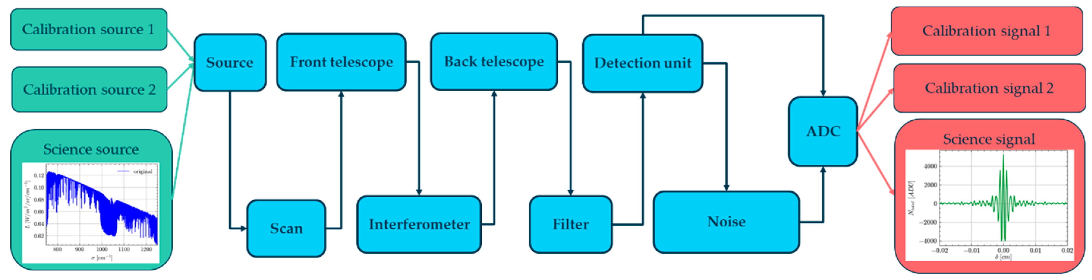
Figure 2.
Instrument schematic. The movement of only one CC is represented in this figure. This sketch was created using the Component Library by Alexander Franzen, licensed under CC BY-NC 3.0.
Figure 2.
Instrument schematic. The movement of only one CC is represented in this figure. This sketch was created using the Component Library by Alexander Franzen, licensed under CC BY-NC 3.0.
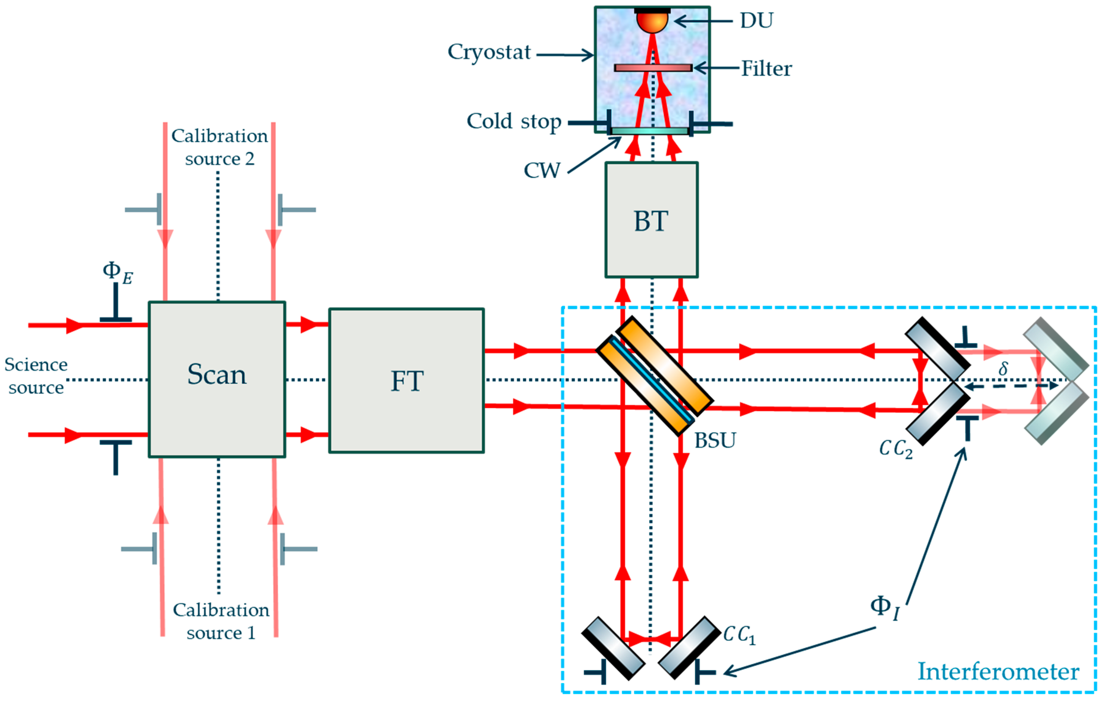
Figure 3.
BSU model with the BP and the CP respectively divided into (P1, P2) and (P3, P4) and the BS at the centre. This sketch was created using the Component Library by Alexander Franzen, licensed under CC BY-NC 3.0.
Figure 3.
BSU model with the BP and the CP respectively divided into (P1, P2) and (P3, P4) and the BS at the centre. This sketch was created using the Component Library by Alexander Franzen, licensed under CC BY-NC 3.0.
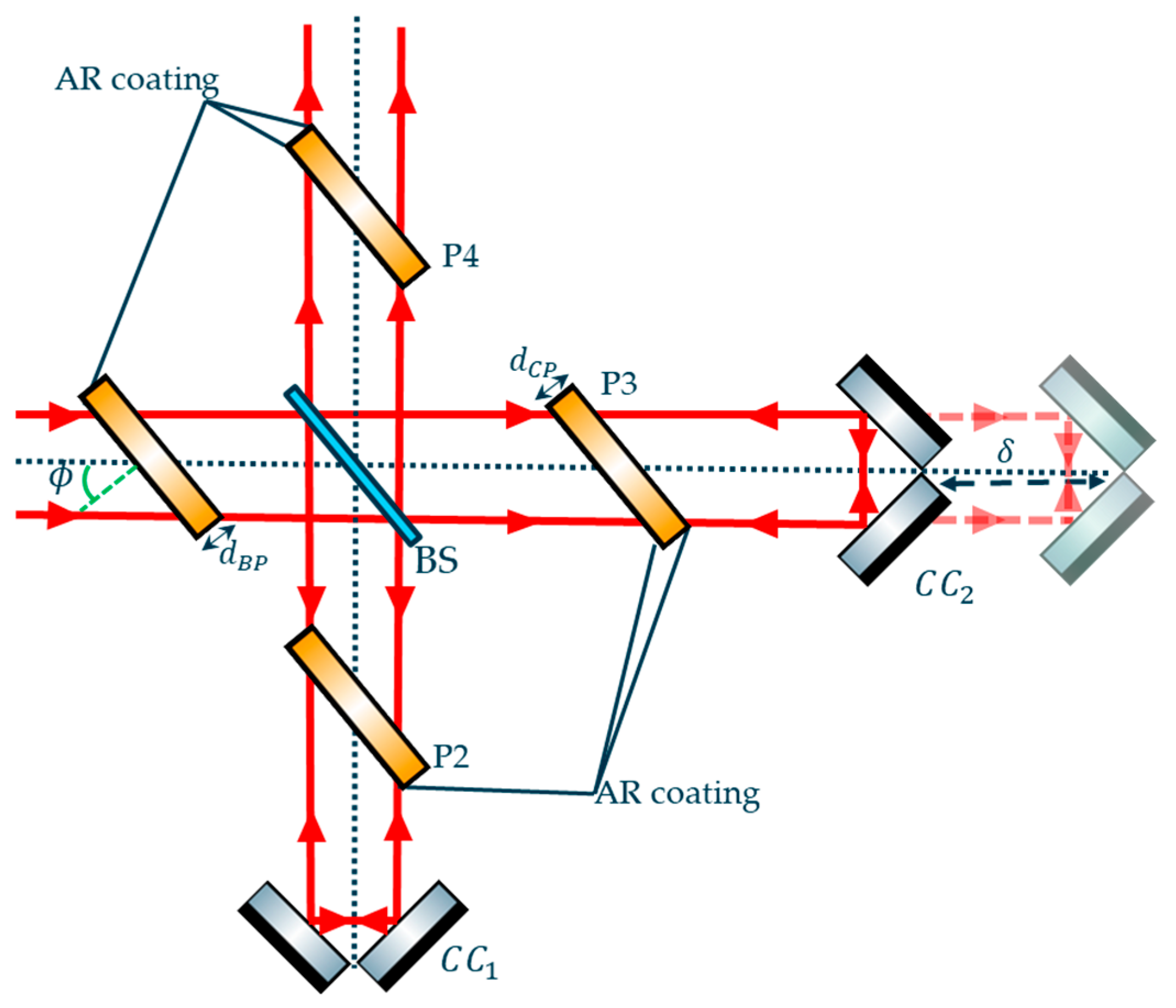
Figure 4.
Photonic and digitized signals. Left panel: Decomposition of photonic signal (red) into source (cyan), thermal background (blue) and dark signal (dashed green) before detector sampling. Right panel: Sampled digitized signal.
Figure 4.
Photonic and digitized signals. Left panel: Decomposition of photonic signal (red) into source (cyan), thermal background (blue) and dark signal (dashed green) before detector sampling. Right panel: Sampled digitized signal.
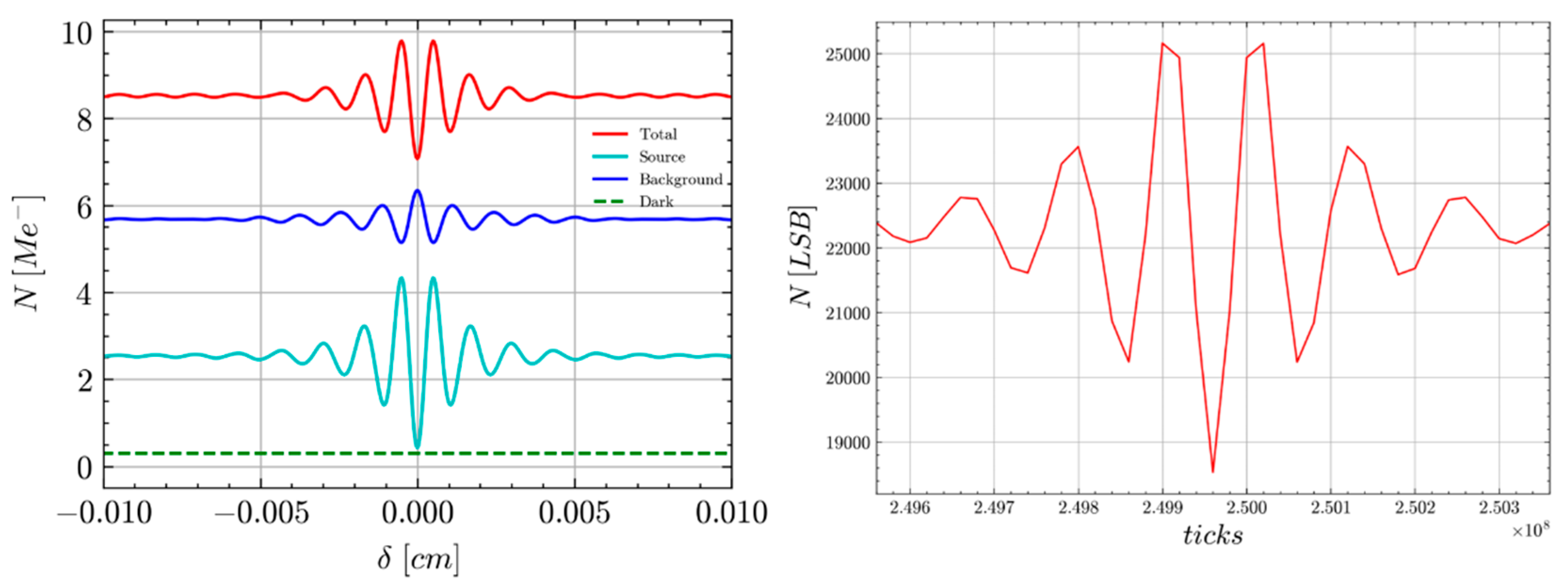
Figure 5.
Layout of thermal background flux emitted from the scan mirror to the filter, with a distinction between the DC flux (red), AC balanced flux (full green) and AC unbalanced (dashed green).
Figure 5.
Layout of thermal background flux emitted from the scan mirror to the filter, with a distinction between the DC flux (red), AC balanced flux (full green) and AC unbalanced (dashed green).
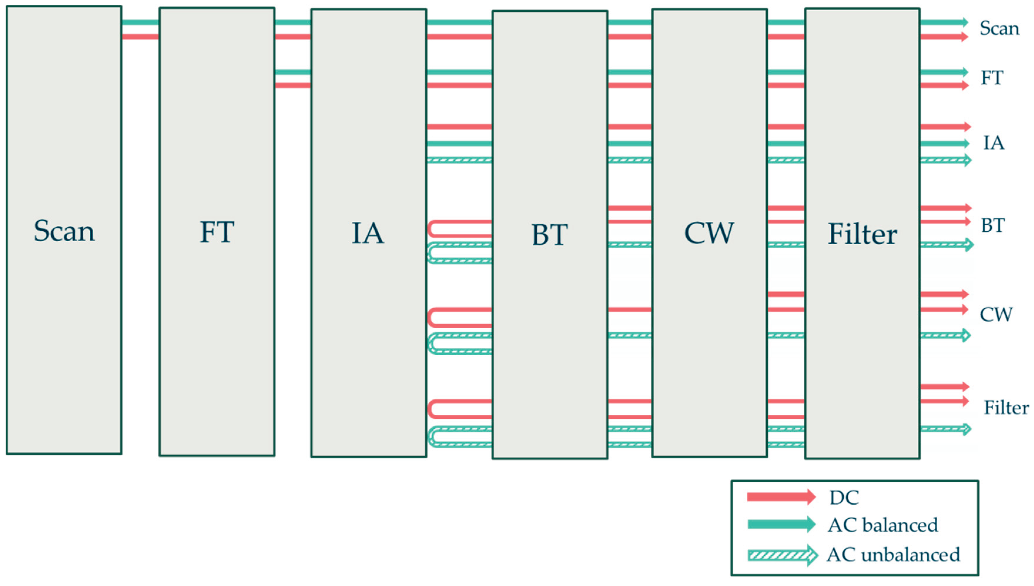
Figure 6.
Effect of self-apodisation on GLORIA at σ = 1400 cm-1 on focal plane irradiance distribution of angular dimension equal to 70.9 × 26.6 mrad2 at 8 cm MOPD (left panel) and the spectral response at a pixel of coordinate (13.3 mrad; 35.4 mrad) (right panel).
Figure 6.
Effect of self-apodisation on GLORIA at σ = 1400 cm-1 on focal plane irradiance distribution of angular dimension equal to 70.9 × 26.6 mrad2 at 8 cm MOPD (left panel) and the spectral response at a pixel of coordinate (13.3 mrad; 35.4 mrad) (right panel).
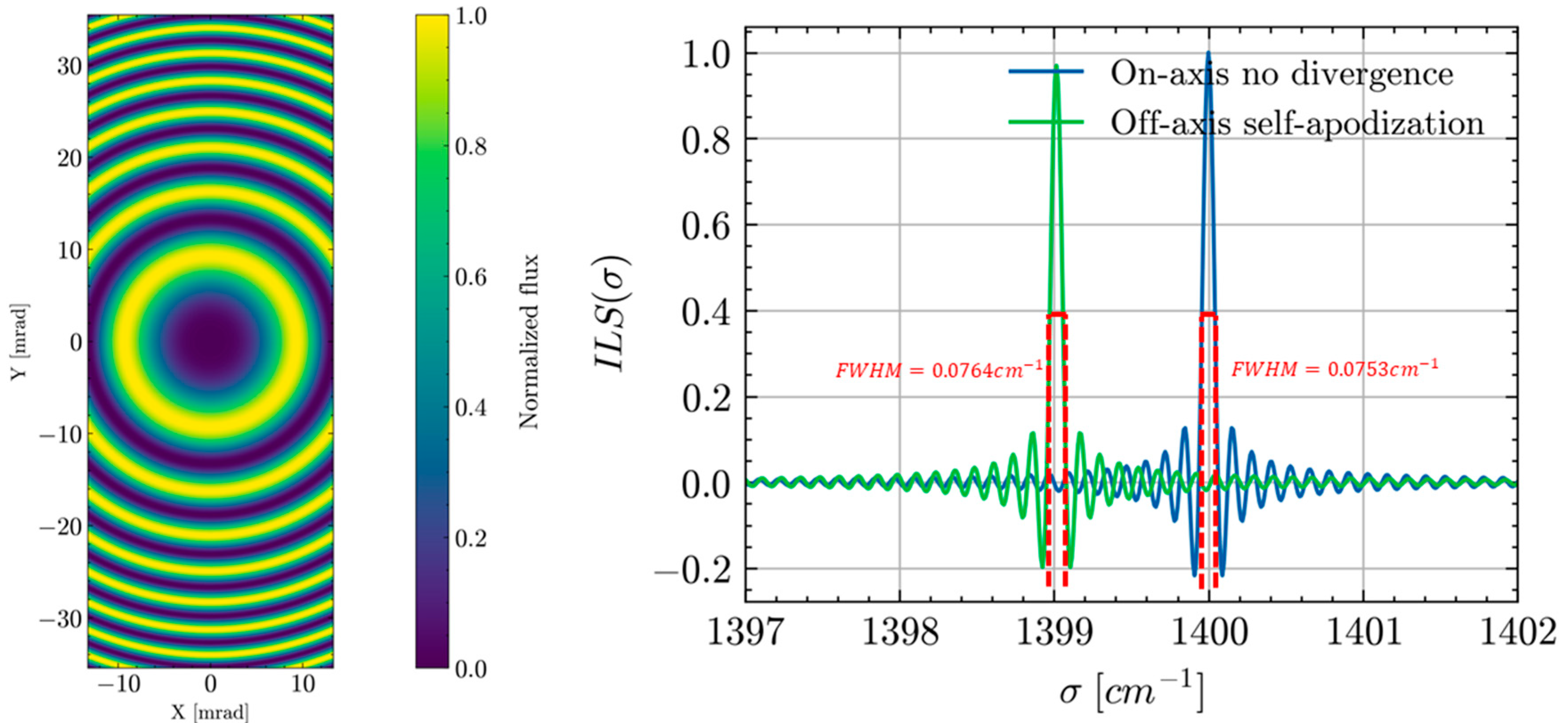
Figure 7.
Inverse model architecture.
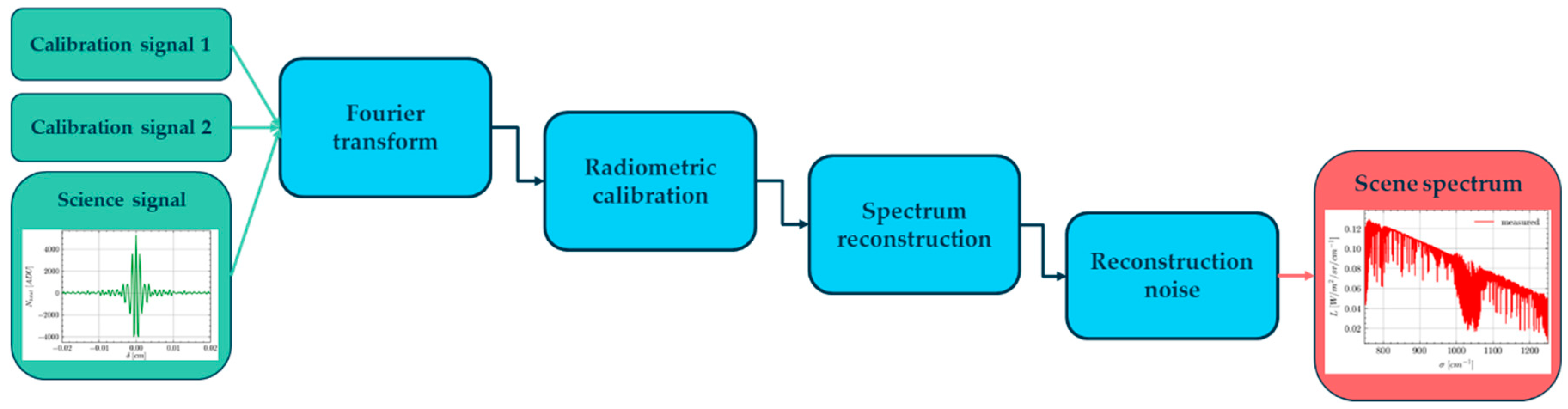
Figure 8.
GLORIA-Lite spectrometer. Left panel: Instrument during its integration phase in Kiruna in 2024. Right panel: Instrument model setup of GLORIA-Lite. This sketch was created using the Component Library by Alexander Franzen, licensed under CC BY-NC 3.0.
Figure 8.
GLORIA-Lite spectrometer. Left panel: Instrument during its integration phase in Kiruna in 2024. Right panel: Instrument model setup of GLORIA-Lite. This sketch was created using the Component Library by Alexander Franzen, licensed under CC BY-NC 3.0.
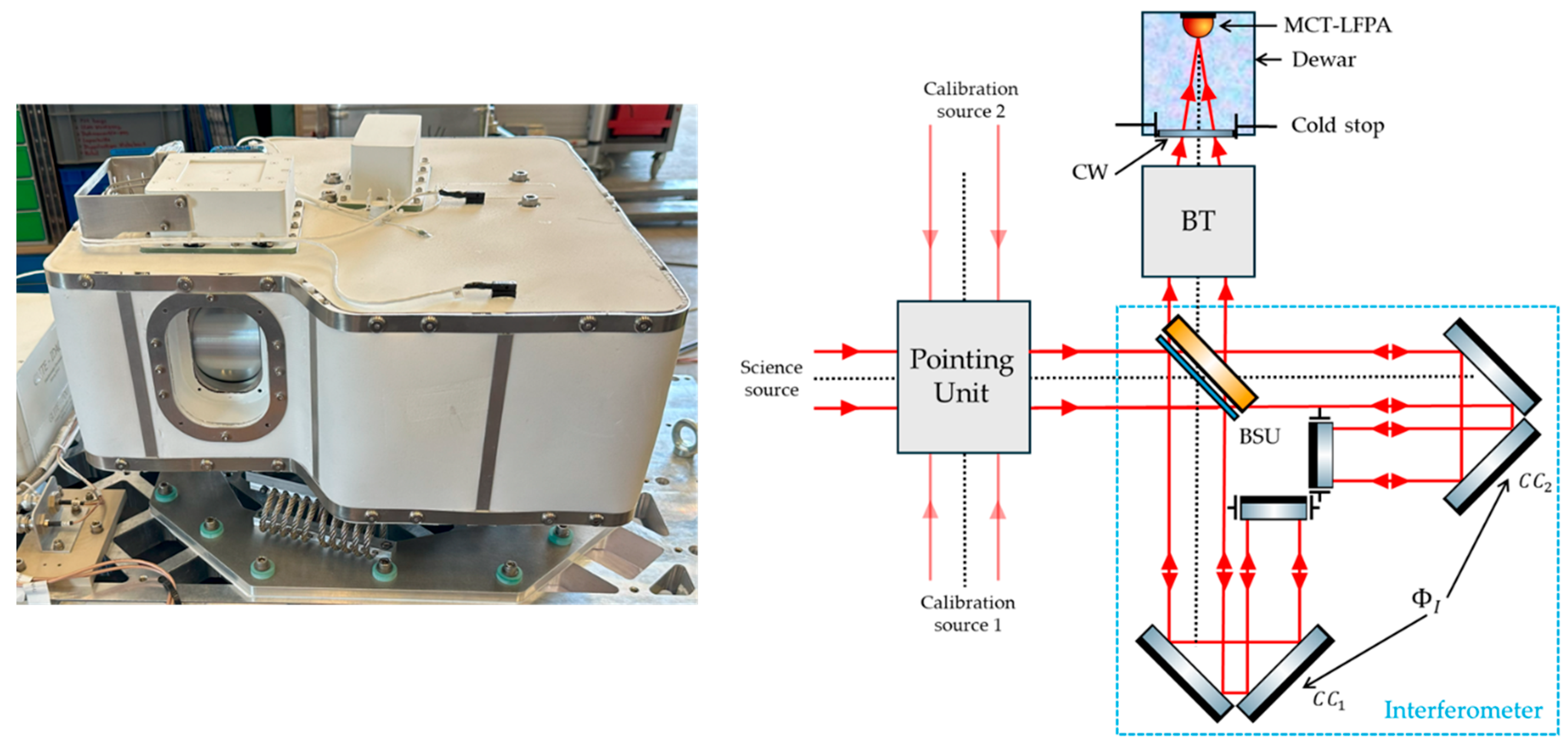
Figure 9.
Illustration of the baseline signal estimation as the average first 2000 frames signal.
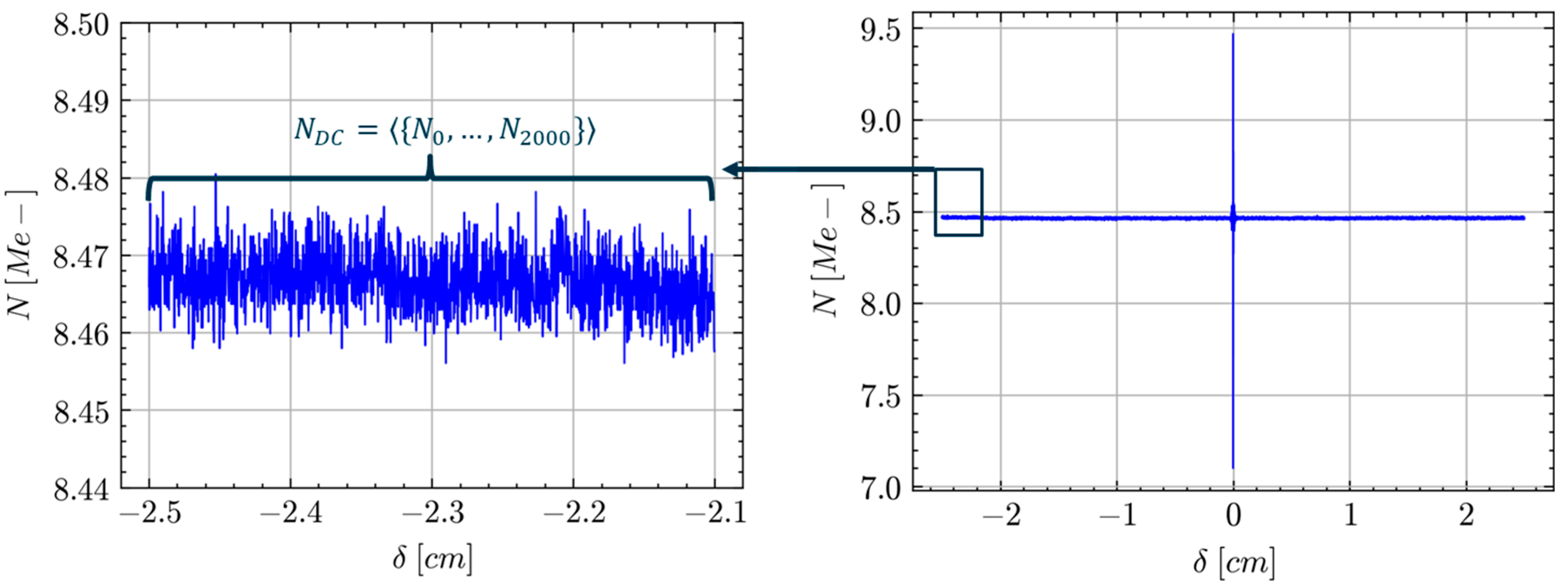
Figure 10.
Contribution of the dark current (dashed green), the atmospheric residuals (cyan) and the instrument thermal background (blue) to the predicted total signal of a deep space acquisition.
Figure 10.
Contribution of the dark current (dashed green), the atmospheric residuals (cyan) and the instrument thermal background (blue) to the predicted total signal of a deep space acquisition.
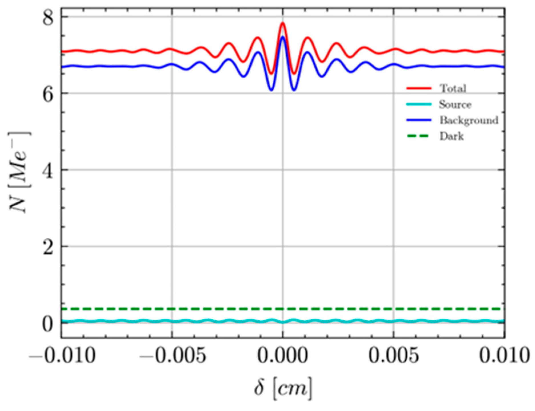
Figure 11.
Model predictions (red) and in-flight measurements (blue) of GLORIA-Lite deep space signals. Left panel: Central pixel signal. Centre panel: Histogram of GLORIA DC level over the detector. Right panel: Histogram of GLORIA ZPD level over the detector.
Figure 11.
Model predictions (red) and in-flight measurements (blue) of GLORIA-Lite deep space signals. Left panel: Central pixel signal. Centre panel: Histogram of GLORIA DC level over the detector. Right panel: Histogram of GLORIA ZPD level over the detector.
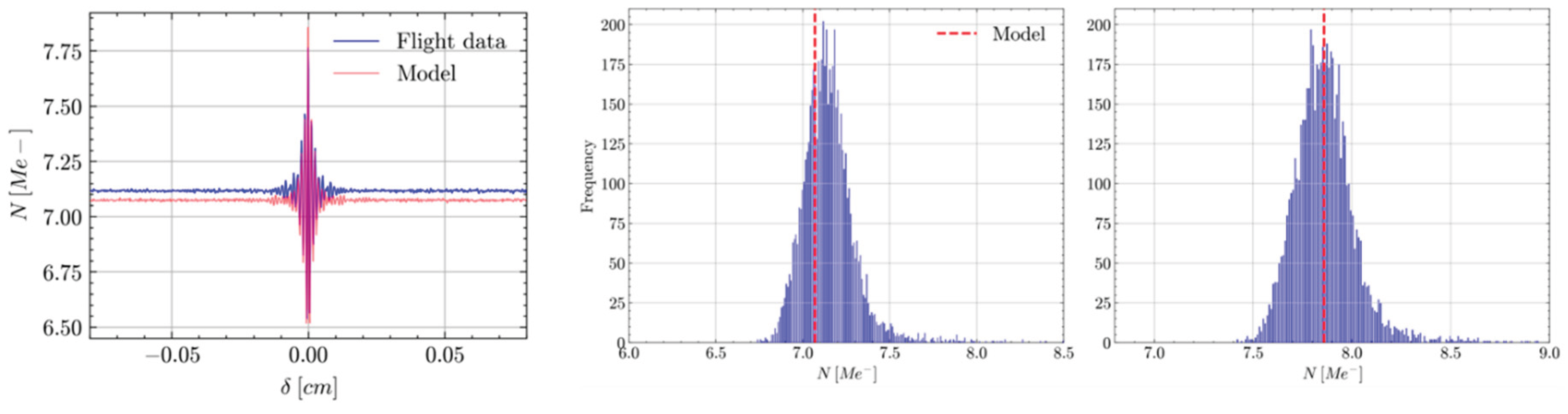
Figure 12.
Model predictions (red) and in-flight measurements (blue) of GLORIA-Lite blackbody signals. Left panel: Central pixel signal. Centre panel: Histogram of GLORIA DC level over the detector. Right panel: Histogram of GLORIA ZPD level over the detector.
Figure 12.
Model predictions (red) and in-flight measurements (blue) of GLORIA-Lite blackbody signals. Left panel: Central pixel signal. Centre panel: Histogram of GLORIA DC level over the detector. Right panel: Histogram of GLORIA ZPD level over the detector.
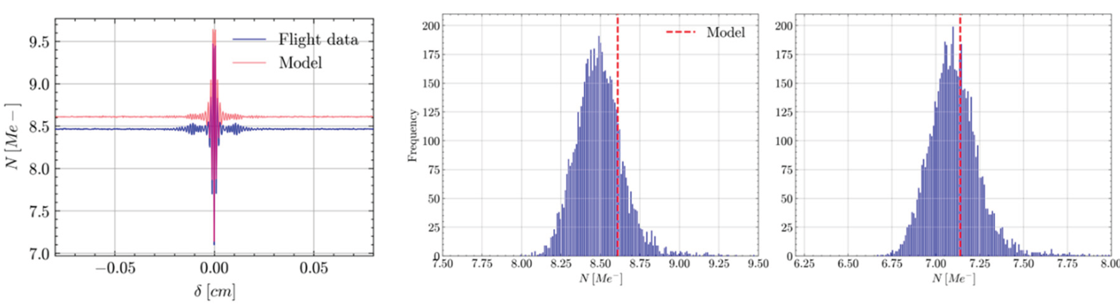
Figure 13.
Model prediction (red) and in-flight measurements (blue) of GLORIA-Lite radiometric calibration outputs at the central pixel. Left panel: Gain magnitude. Right panel: Offset real part.
Figure 13.
Model prediction (red) and in-flight measurements (blue) of GLORIA-Lite radiometric calibration outputs at the central pixel. Left panel: Gain magnitude. Right panel: Offset real part.
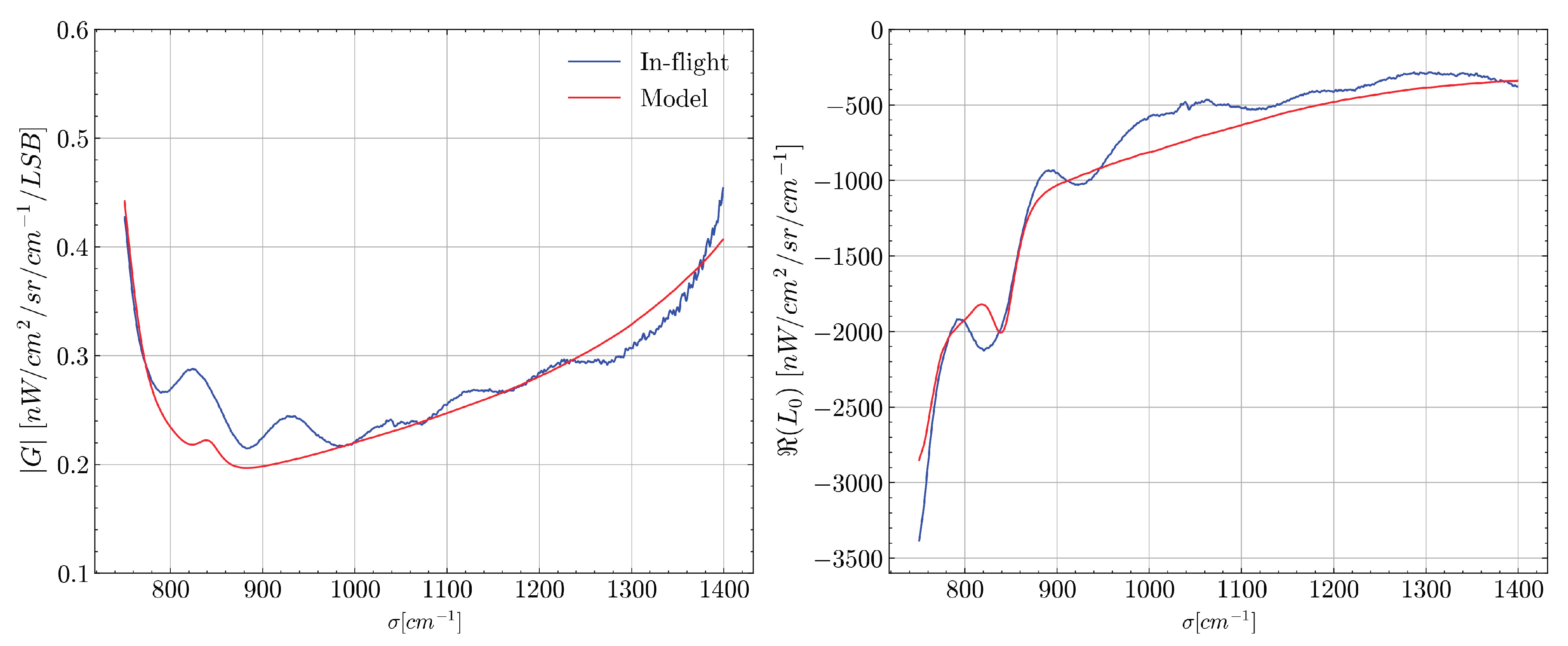
Figure 14.
Limb reference scene reconstruction at 0.385 cm-1 apodized resolution (green) versus the “original” spectrum at 0.050 cm-1 resolution (magenta). A zero-filling up to 218 points and a Norton-Beer strong apodisation have been applied on the interferograms. Top-left panel: Global view from 780 cm-1 to 1400 cm-1. Top-right panel: Zoomed view between 790 cm-1 and 800 cm-1. Bottom left panel: Zoomed view between 945 cm-1 and 955 cm-1. Bottom right panel: Zoomed view between 1360 cm-1 and 1370 cm-1.
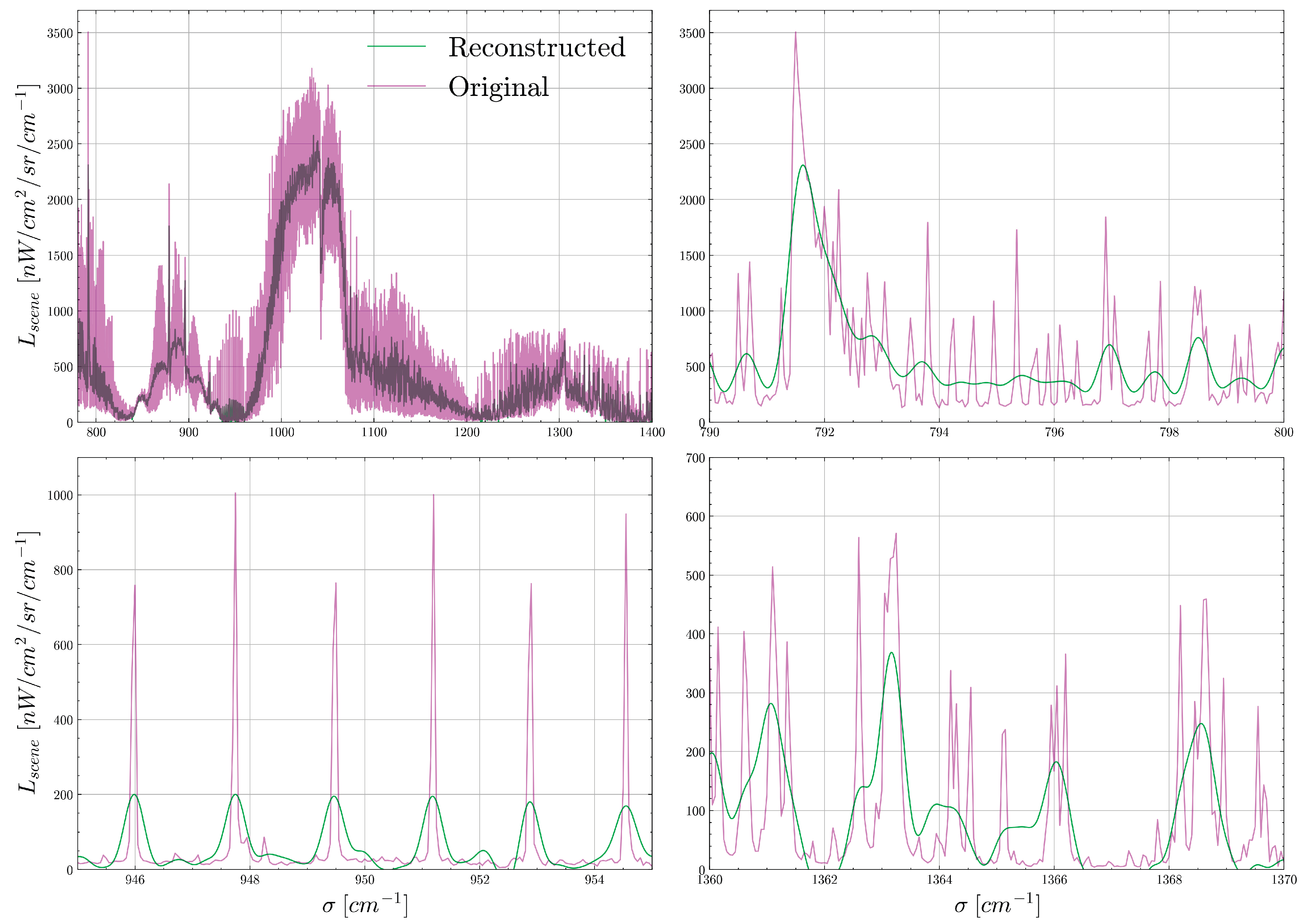
Figure 15.
Theoretical spectrum (right panel) obtained as the convolution of the “original” spectrum (left panel) with the ILS (middle panel), considering a Norton-Beer strong apodisation.
Figure 15.
Theoretical spectrum (right panel) obtained as the convolution of the “original” spectrum (left panel) with the ILS (middle panel), considering a Norton-Beer strong apodisation.
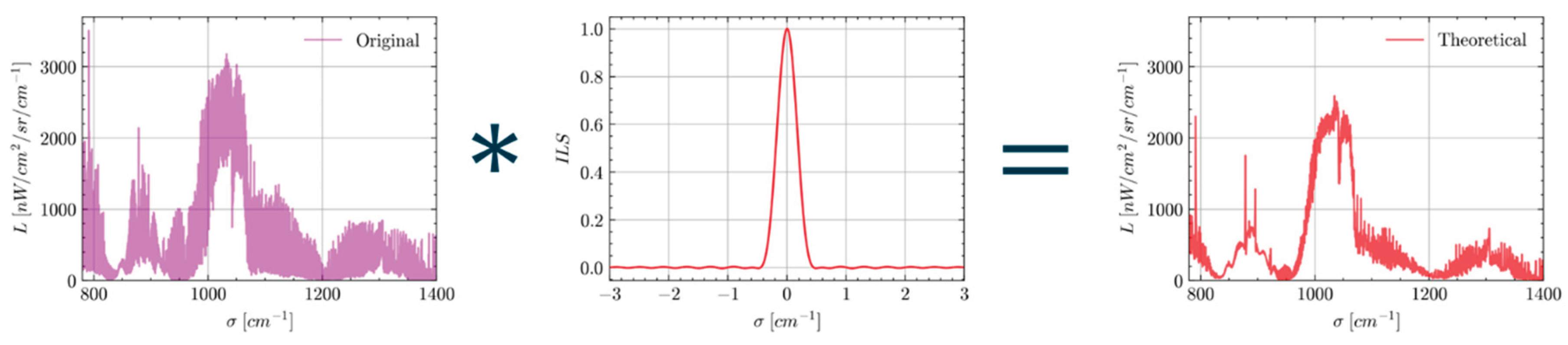
Figure 16.
Comparison between the inverse model (green) and the theoretical (dashed red) noiseless spectral radiances at 0.385 cm-1 apodised resolution. The theoretical spectrum is obtained by the convolution of the input spectrum with the ILS and considering a Norton-Beer strong apodisation. Left panel: View between 790 cm-1 and 800 cm-1. Middle panel: View between 945 cm-1 and 955 cm-1. Right panel: View between 1360 cm-1 and 1370 cm-1.
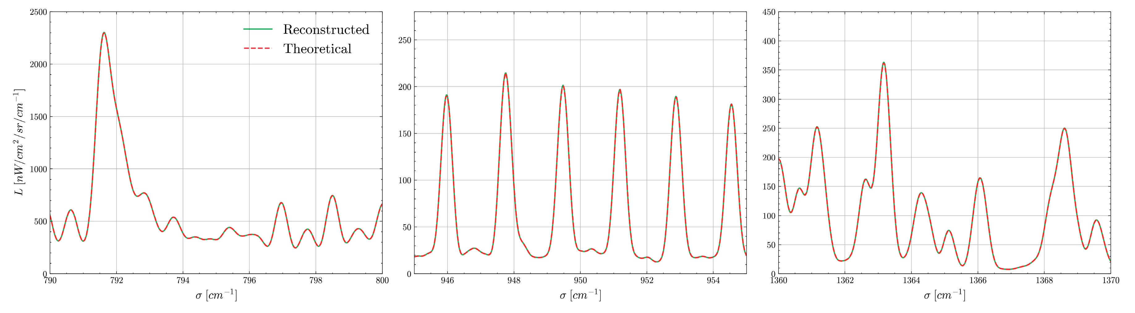
Table 1.
Comparison between ESA and state of the art FTS models extracted from literature: inputs, workflow and outputs of each model. A green-filled tick indicates a capability, a pink-filled cross marks a feature that is not included, and a yellow minus sign denotes an effect that is only partially modelled or could be incorporated with limited-effort update.
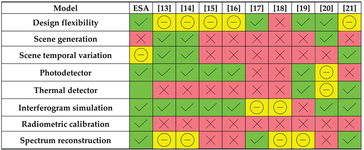 |
Table 2.
Comparison between ESA and state of the art literature FTS models: Instrumental effects and errors.
Table 2.
Comparison between ESA and state of the art literature FTS models: Instrumental effects and errors.
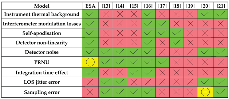 |
Table 4.
Error budget on the baseline and ZPD signals on a blackbody acquisition.
| Contributors | ΔNDC / NDC % | ΔNZPD / NZPD % | Precision |
| Optics Temperature | 0.67 % | 0.90 % | 0.5 K |
| Dark current | 0.02 % | 0.03 % | 2.16 mA/m2 |
| PRNU | 1.95 % | 1.94 % | 2% |
| blackbody emissivity | 0.09 % | 0.17 % | 0.003 |
| blackbody temperature | 0.02 % | <0.01 % | 0.03 K |
| Mirrors reflectivity | 0.64 % | 1.00 % | 0.0005 |
| BS transmission | <0.01 % | 0.01 % | 0.005 |
| BP optical thickness | 0.05 % | 0.14 % | 0.05 mm |
| BP AR coating reflectivity | 0.21 % | 0.16 % | 0.0005 |
| Total | 2.17 % | 2.37 % | - |
Disclaimer/Publisher’s Note: The statements, opinions and data contained in all publications are solely those of the individual author(s) and contributor(s) and not of MDPI and/or the editor(s). MDPI and/or the editor(s) disclaim responsibility for any injury to people or property resulting from any ideas, methods, instructions or products referred to in the content. |
© 2025 by the authors. Licensee MDPI, Basel, Switzerland. This article is an open access article distributed under the terms and conditions of the Creative Commons Attribution (CC BY) license (http://creativecommons.org/licenses/by/4.0/).
Copyright: This open access article is published under a Creative Commons CC BY 4.0 license, which permit the free download, distribution, and reuse, provided that the author and preprint are cited in any reuse.