Submitted:
24 August 2025
Posted:
25 August 2025
You are already at the latest version
Abstract
Neural representations can be modelled as probability distributions that evolve over time.Understanding how these distributions transform among brain regions remains a fundamentalchallenge within computational neuroscience. We introduce a framework that characterizessuch transformations in terms of gradient flows — dynamical trajectories that follow thesteepest ascent of two information-theoretic functionals given by entropy and expectation. Weshow that these two functionals account for orthogonal flows in the case of Gaussiandistributions. Furthermore, the linear combination of entropy and expectation allows for thedecomposition of neural transformations into interpretable components. We first validate thisframework in silico by demonstrating robust recovery of the gradient flows from observablesignal features. We then apply the same framework to two-photon imaging data collected frommurine visual cortex. We identify consistent flow between the rostrolateral area and primaryvisual cortex across all five mice, indicating a bi-directional mapping of the neural activitypatterns between these two cortical regions. Our approach offers a generalizable method thatcan be used to separate information-theoretic flows, not just among brain regions, but alsoacross neuroimaging modalities and observational scales.
Keywords:
mouse
; visual cortex
; information theory
Introduction
The electrical activity in the brain reflects a combination of hidden internal states which, although not directly observable, can be inferred via the signals picked up by neuroimaging devices [1-3]. One way to describe these signals is in terms of probability distributions evolving in time. As conditions change in the brain, the probability distributions shift accordingly, reflecting an ongoing reorganization of internal representations. Understanding precisely how these distributions evolve, and what computational processes underlie their transformations among brain regions, remains a central challenge in computational neuroscience.
Changes in neural activity can be analysed by studying how specific functionals act on probability distributions. Two key examples of such functionals are entropy[4-6], which affects the variance, and expectation[7-9], which shifts the mean. Each functional is associated, via its gradient, with a specific flow across the space of probability densities. This geometric[10] perspective allows for a decomposition of transformations into interpretable information-theoretic components.
We specifically formulate the change in probability distributions when the observation scale is altered. This perspective also aligns with established computational theories such as predictive coding[11,12] and efficient representation[13-15], in which internal states are continuously adjusted to balance precision and uncertainty. By framing representational change as a gradient flow, we model these adjustments as structured, directional transformations shaped by information-theoretic drives.
Previous work on neural signal transmissions has largely focused on statistical dependencies between observed activation patterns[16,17] — whether scalar (e.g., firing rates) or vector-valued (e.g., population activity). Metrics such as mutual information[18,19] and Granger causality[20] quantify how strongly activity in one region predicts activity in another. However, these metrics do not capture how the full probability distributions over latent variables are transformed across regions. We address precisely this issue with a framework that quantifies the form of gradient flows over probability distributions. We then show that entropy and expectation form orthogonal flows in the case of Gaussian distributions.
We validate this framework in silico and then extract dominant flows linking regions within the murine visual cortex, captured using two-photon imaging. The visual cortex in mice is particularly well-suited to our study, given that adjacent cortical regions therein exhibit coordinated patterns of activity[21,22] across functionally specialized regions[23-25]. Beyond this specific application, our approach introduces a generalizable method for analysing any scenario in which distributions are transformed — not just among cortical regions, but also between measurement devices, or across spatiotemporal scales.
Methods
Our goal is to derive orthogonal gradient directions of a probability distribution with respect to changes in observational scale. These gradients indicate the directions along which the distribution undergoes maximal change. We begin with the following definitions:
:the state of the system, represented by an -dimensional variable.
:a positive-valued parameter that controls the scale of observation.
: a probability density function over , conditioned on the observation scale , which remains normalized for all values of , such that:
We define the space of all valid (smooth, positive, normalized) probability distributions as information space :
This defines a nonlinear manifold of valid distributions within the space of all possible functions.
Power law generators: Due to the ubiquity of power laws in the analysis of neural systems2, we investigate how the probability distribution changes to a new distribution via:
where the partition function in the denominator ensures correct normalization of the new distribution for all values of .
We next analyse the form of Eq. for very small changes in scale. Specifically, we seek the associated generator[26] — i.e., the infinitesimal power law transformation associated with an increase in . As motivated by Noether’s theorem[27] and Lie theory[28], the derivation of a generator creates a powerful tool that allows for the recovery of arbitrary transformations.
To see how this applies to our case, we begin by defining the scale parameter in terms of an arbitrarily small constant :
thereby allowing for any scale parameter to be defined by the iterated application of .
Applying Eq. to Eq. , we obtain:
Next, using the fact that for small , we then expand to first order in and use the identities: , and , to linearize the effect of a power law transform:
which defines the transformation from Eq. evaluated near .
To ensure that the transformed density remains normalized, we divide Eq. (4) by its associated partition function:
Substituting the normalization condition from Eq. into the denominator, and using the definition of the mean:
Eq. simplifies to:
Finally, we use the fact that for small and to linearize Eq. , thereby yielding the power law generator:
which can equivalently be expressed as the following differential equation:
Power law and Entropic Flow: We now note that the generator derived in Eq. includes a term , which resembles the integrand of entropy , hinting at a connection between power law transformations and entropy:
We investigate this connection by calculating in which direction, within the space of valid probability distributions in Eq. , entropy increases most rapidly.
This direction is given by the (negative) functional gradient of the entropy in Eq. :
with a mean given by:
which, using Eqs. and , can be written as:
We define an entropic flow as the mean gradient in Eq. subtracted from the gradient in Eq. . This has the effect of projecting the gradient onto the manifold of valid probability densities in Eq. :
which, using Eqs. and , reads:
i.e., we discover exactly the same expression as in Eq. , meaning that we can write:
This reveals a relationship between entropic flow and power law transformations indexed by a scale parameter .
Generalized Flow: The form of Eq. can be generalized to arbitrary functionals , which define continuous trajectories through information space via associated flow parameters . The flow of preserves the geometric structure of Eq. , in terms of a projected gradient on the log density of , while allowing for arbitrary functionals:
Here, the term is not an artefact of the entropic expression in Eq. . Rather, persists in the generalized flow expression in Eq. because parameterizes a flow of the form , which maps to . Eq. therefore yields a class of projected gradient flows which depend on the choice of functional .
Basis Flows: Thus far we have established that:
- Power law transformations are associated with entropic flow,
- The power law/entropy link can be generalized to arbitrary functionals other than entropy.
Given the above two points, our next question is whether we can find a flow that is orthogonal to entropic flow , as this would allow for a decomposition into independent components. To find such an orthogonal flow, we require that the inner product between and equals zero:
where we can use Eqs. and to write the covariance as:
which is equivalent to the covariance between and under :
The simplest class of is given by linear expectation:
with a functional derivative given by:
If we then assume a Gaussian form for , for which , Eq. becomes:
which satisfies the orthogonality condition in Eq. , which in turn shows that entropy and expectation define orthogonal flows under the zero-mean Gaussian distribution. It is important to note that this orthogonality only holds for symmetric distributions.
We next look for the transformation associated with the expectation functional using Eq. :
which has a solution given by:
and hence:
where the partition function in the denominator ensures correct normalization.
Therefore, just as entropic flow arises from power law transformations in Eq. , the expectation flow corresponds to an exponential tilt in Eq. . Intuitively, the entropic and expectation flows capture how variance and expectation change with observational scale, respectively. We can summarize the links between these two information-theoretic functionals and their associated geometric transformations as follows:
Entropic flow:
- Functional: Entropy:
- Flow: Entropic gradient ascent:
- Transformation:Power law re-weighting:
Expectation flow:
- Functional: Expectation value :
- Flow: Expectation gradient ascent:
- Transformation: Exponential tilt:
Synthetic Data: Having established entropy and expectation as orthogonal basis functionals, we now consider a mixed entropic-expectation via Eqs. and :
where the parameters and determine the relative contributions of entropy and expectation, respectively.
We performed two in silico tests to validate parameter recovery. We simulated the flow in Eq. using pre-specified values of the entropy () and expectation () coefficients, using samples from: 1) a Gaussian process and 2) a one-dimensional Langevin process with a time-varying oscillatory drift term. In both cases, recovery accuracy for and was assessed by comparing true vs. recovered parameters and evaluating distribution similarity via Wasserstein, total variation, and L2 metrics.
Two-photon imaging data: We then evaluated the relative contribution of the entropy and expectation flows in an empirical dataset. We used publicly available two-photon imaging data collected in five mice[29]. The dataset includes individual neuronal responses collected from six retinotopically defined visual cortical areas: the primary visual cortex (V1), lateromedial (LM), anterolateral (AL), rostrolateral (RL), anteromedial (AM), and posteromedial (PM) areas (see Figure 1).
Visual stimuli consisted of movies with durations of 30–120 seconds, and resting state activity was recorded under a constant grey screen for 5 minutes. All recordings were pre-processed to extract ΔF/F calcium traces and responses from neurons were aligned to stimulus timing and grouped by retinotopically defined visual area (see Figure 2).
We then apply the mixed-flow transformation model in Eq. to all pairs of regions in the visual cortices in the five mice. For each region, we estimate its marginal probability distribution using a 100-bin histogram of its mean time series. Given a pair of regions and , we treat the mean time series of region as the input signal and that of region as the target output. We then use nonlinear optimization to identify the values of and in Eq. that best transform region ’s time series into that of region .
We note that, while Eq. was derived for the transformation of a single distribution under changes in observational scale, the same operator can be used to formalize transformations between the marginal distributions of two regions. Specifically, given regions and with empirical distributions and , we approximate their relationship as:
where denotes the mixed entropic–expectation flow operator defined in Eq. . In this way, the inter-regional transformation is treated as the best-fitting reweighting and tilting of that recovers . This allows the flow coefficients and to be interpreted not only as within-distribution drives, but also as markers of how distributions from different regions are related under the same geometric framework.
The transformation is composed of two components: a nonlinear entropic flow term driven by the deviation of local log-density from its mean, and a linear expectation flow term driven by the deviation from the global mean. These two terms respectively capture how local compressions in probability mass and global shifts in signal level contribute to the transformation. Once the optimal and parameters are obtained for each pair of regions, the input signal is warped accordingly to produce an estimated output signal. The match between the estimated and actual target signals is quantified using the coefficient of determination .
To assess whether each of the transformations are statistically significant, we compare empirical results to null distributions obtained through temporal permutation. To generate null distributions, we circularly shift the input time series independently within each session and re-estimate the transformation parameters. This process is repeated 1000 times with random shift sizes to generate surrogate distributions. These surrogate datasets allow us to compare our empirical results with the null hypothesis that there is a lack of alignment between source and target signals. Significance values are computed as the proportion of surrogate values greater than or equal to the empirical result. These -values are corrected for multiple comparisons using the false discovery rate (FDR, ). Only values that survive FDR correction and exceeded a conservative threshold of are reported.
Results
All results can be reproduced with the accompanying code (see Code Availability).
Synthetic data: We created two forward-generative models using known entropy and expectation flow parameters from Eq. : 1) a Gaussian process undergoing noise-driven diffusion (Figure 3A); and 2) a stochastic Langevin process with a sinusoidal drift (Figure 3B).
(red) and at a later point in time (black). The solid and dashed lines indicate the distributions generated with ground-truth and recovered parameters, respectively. B)A signal x(t) evolves according to a stochastic Langevin process with an oscillatory drift using ground-truth (red) and recovered (black) para-meters.
In the case of the Gaussian process (Figure 3A), the model recovered and with errors of 24.4% and 19.8%, respectively. The recovered distributions accurately matched the ground-truth distributions across time, with an average squared Wasserstein-2 distance of , a total variation distance of , and a mean error of .
In the case of the Langevin process (Figure 3B), the recovered and values deviated from the ground-truth values by 7.1% and 3.0%, respectively. The recovered signal closely tracked the ground-truth trajectory, with a total variation distance of 0.02 and an error of 0.03.
Empirical data: We computed the first principal component of pixel activity within each region of the visual cortex and used the mixed-flow transformation from Eq. to model signals within one region, based on another region’s activity. We show an example of using the primary visual cortex (V1) to estimate the anteromedial area (AM) (, Figure 4).
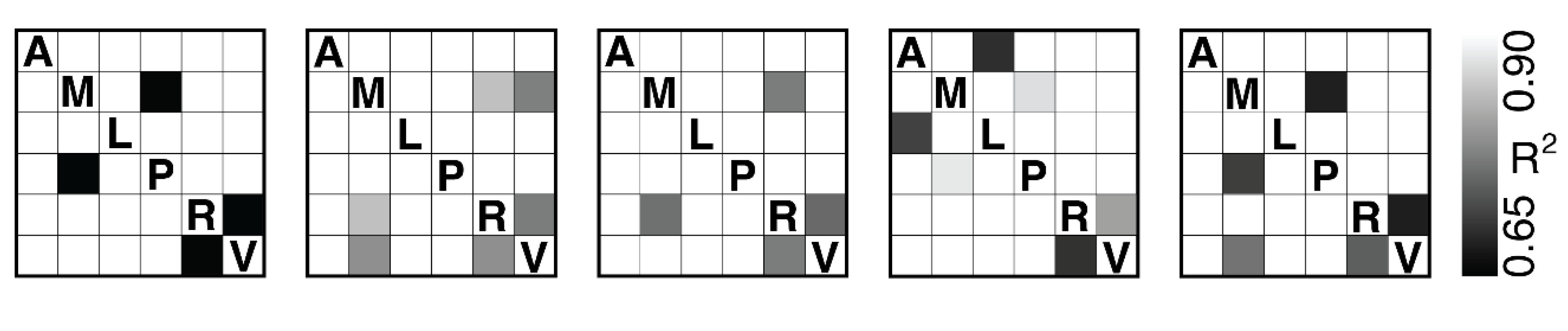
We performed this same analysis for every pair of regions across mice. The bi-directional connections between the rostrolateral cortex (RL) and the primary visual cortex (V1) were the only links surviving false discovery rate (FDR) correction and exceeding a threshold of across all five mice (Figure 5).
Discussion
In this study, we formalize the link between the geometric structure of probability distributions and their information-theoretic content. Specifically, we show that transformations between Gaussian probability distributions can be decomposed into orthogonal entropic and expectation-based components. We validated this framework on synthetic data, first with a noise-corrupted diffusing Gaussian distribution, and then with a one-dimensional Langevin process with a time-varying oscillatory drift. We then applied the methodology to empirical timeseries obtained from two-photon neuroimaging data collected in the murine visual cortex.
Our analysis of the neuroimaging data revealed a robust bi-directional transformation between the neural probability distributions derived from the rostrolateral area (RL) and the primary visual cortex (V1). These transformations exceeded an threshold of 0.65 across all five mice after false discovery rate (FDR) correction. This finding indicates that information-theoretic relationships are preserved between the distributions produced by RL and V1. This reciprocity enables coordination between regions responsible for early sensory processing (V1) and higher-order contextual integration (RL)[30,31].
The RL region in mice integrates visual input from V1 with signals related to movement and task demands[32]. In this regard, RL plays a functional role analogous to the parietal cortex in primates, facilitating visuomotor coordination[33]. The bi-directional transformations observed between RL and V1 indicate a shared encoding of information between the two regions. V1 acts as a primary sensory area providing input to RL, which in turn serves as a higher-order region that modulates V1. This recurrent loop aligns with predictive coding theories, which propose that visual processing relies on a reciprocal interaction between brain regions and across hierarchical levels[34].
The link between neural dynamics and information processing shown here aligns with existing computational theories. For instance, the efficient coding hypothesis proposes that neural systems adapt their responses to match the statistical structure of sensory input[35]. In our framework, entropic and expectation flow achieve this adaptation by adjusting the spread and mean of neural activity distributions to match ongoing conditions. In communication-through-coherence (CTC) models[36], information is most effectively exchanged between two brain regions when the signals from one arrive at moments when the other is most responsive — i.e., when its neurons are closer to firing. In the context of our work, times of unpredictable sensory stimuli are associated with a dominant entropic flow, which in turn increases the range of available signal responses. On the other hand, times of predictable activity during e.g., task focus are associated with a dominant expectation flow, which shifts responses towards relevant signal averages.
Neuroscience studies often employ methods such as Granger causality[37] and mutual information[38] to quantify statistical dependencies between activity in pairs of brain regions. These approaches indicate whether activity in one region predicts activity of another, but they do not specify the form of the transformation linking the two. Our framework addresses this gap by modelling how one region’s probability distribution is geometrically transformed into that of another. The orthogonality of entropic and expectation flows further ensures (under the assumption of Gaussianity) that these transformation components can be interpreted independently.
In summary, we introduce a framework that decomposes information-geometric transformations between neural probability distributions into information-theoretic flow components. We demonstrated this in the murine visual cortex. However, the approach is applicable to any system from which probability distributions can be estimated. For example, it can be used to characterise transformations between different neuroimaging modalities, revealing scale-dependent aspects of neural organisation. Alternatively, our methodology can be used to detect disease progression, for instance in disrupted network coordination in epilepsy[39] or in altered representational scaling in Alzheimer’s disease[40]. By linking geometric transformations directly to information-theoretic content, our framework provides a versatile method for testing theories of neural function across species, modalities, and scales.
Supplementary Materials
The following supporting information can be downloaded at the website of this paper posted on Preprints.org.
Funding
The authors acknowledge support from Masaryk University and project nr. LX22NPO5107 (MEYS): Financed by European Union – Next Generation EU. E.D.F. was supported by the Czech Health Research Agency (AZV, NW25-04-00226). H.T. was supported by Grant-in-Aid for Scientific Research (C) (22H05079, 22H05082, 25K14517), the Japan Society for the Promotion of Science, and Japan Science and Technology Agency (JST), CREST Grant Number JPMJCR2433.
Code Availability
All MATLAB code used to produce results is made available at: https://github.com/allavailablepubliccode/info_flow
Data Availability Statement
All data used are available in the following repository: https://figshare.com/articles/dataset/Data_from_Functional_Parcellation_of_Mouse_Visual_Cortex_Using_Statistical_Techniques_Reveals_Response-Dependent_Clustering_of_Cortical_Processing_Areas_/13476522/1
References
- Ma, W.J.; Beck, J.M.; Latham, P.E.; Pouget, A. Bayesian inference with probabilistic population codes. Nat. Neurosci. 2006, 9, 1432–1438. [Google Scholar] [CrossRef]
- Fiser, J.; Berkes, P.; Orbán, G.; Lengyel, M. Statistically optimal perception and learning: from behavior to neural representations. Trends Cogn. Sci. 2010, 14, 119–130. [Google Scholar] [CrossRef] [PubMed]
- Friston, K. A theory of cortical responses. Philosophical transactions of the Royal Society B: Biological sciences 2005, 360, 815–836. [Google Scholar] [CrossRef]
- Fagerholm, E.D.; Dezhina, Z.; Moran, R.J.; Turkheimer, F.E.; Leech, R. A primer on entropy in neuroscience. Neurosci. Biobehav. Rev. 2023, 105070. [Google Scholar] [CrossRef]
- Keshmiri, S. Entropy and the brain: An overview. Entropy 2020, 22, 917. [Google Scholar] [CrossRef]
- Luczak, A. Entropy of Neuronal Spike Patterns. Entropy 2024, 26, 967. [Google Scholar] [CrossRef]
- Gerstner, W.; Kistler, W.M. Spiking neuron models: Single neurons, populations, plasticity; Cambridge university press: 2002.
- Lánský, P.; Sacerdote, L. The Ornstein–Uhlenbeck neuronal model with signal-dependent noise. Phys. Lett. A 2001, 285, 132–140. [Google Scholar] [CrossRef]
- Helias, M.; Tetzlaff, T.; Diesmann, M. The correlation structure of local neuronal networks intrinsically results from recurrent dynamics. PLoS computational biology 2014, 10, e1003428. [Google Scholar] [CrossRef]
- Nielsen, F. The many faces of information geometry. Not. Am. Math. Soc 2022, 69, 36–45. [Google Scholar] [CrossRef]
- Rao, R.P.; Ballard, D.H. Predictive coding in the visual cortex: a functional interpretation of some extra-classical receptive-field effects. Nat. Neurosci. 1999, 2, 79–87. [Google Scholar] [CrossRef]
- Clark, A. Whatever next? Predictive brains, situated agents, and the future of cognitive science. Behav. Brain Sci. 2013, 36, 181–204. [Google Scholar] [CrossRef]
- Barlow, H.B. Possible principles underlying the transformation of sensory messages. Sensory communication 1961, 1, 217–233. [Google Scholar]
- Simoncelli, E.P.; Olshausen, B.A. Natural image statistics and neural representation. Annu. Rev. Neurosci. 2001, 24, 1193–1216. [Google Scholar] [CrossRef]
- Wei, X.-X.; Stocker, A.A. A Bayesian observer model constrained by efficient coding can explain'anti-Bayesian'percepts. Nat. Neurosci. 2015, 18, 1509–1517. [Google Scholar] [CrossRef]
- Friston, K.J. Functional and effective connectivity: a review. Brain Connect. 2011, 1, 13–36. [Google Scholar] [CrossRef] [PubMed]
- Bastos, A.M.; Schoffelen, J.-M. A tutorial review of functional connectivity analysis methods and their interpretational pitfalls. Front. Syst. Neurosci. 2016, 9, 175. [Google Scholar] [CrossRef]
- Borst, A.; Theunissen, F.E. Information theory and neural coding. Nat. Neurosci. 1999, 2, 947–957. [Google Scholar] [CrossRef]
- Panzeri, S.; Harvey, C.D.; Piasini, E.; Latham, P.E.; Fellin, T. Cracking the neural code for sensory perception by combining statistics, intervention, and behavior. Neuron 2017, 93, 491–507. [Google Scholar] [CrossRef]
- Seth, A.K.; Barrett, A.B.; Barnett, L. Granger causality analysis in neuroscience and neuroimaging. J. Neurosci. 2015, 35, 3293–3297. [Google Scholar] [CrossRef]
- Harris, J.A.; Mihalas, S.; Hirokawa, K.E.; Whitesell, J.D.; Choi, H.; Bernard, A.; Bohn, P.; Caldejon, S.; Casal, L.; Cho, A. Hierarchical organization of cortical and thalamic connectivity. Nature 2019, 575, 195–202. [Google Scholar] [CrossRef]
- Felleman, D.J.; Van Essen, D.C. Distributed hierarchical processing in the primate cerebral cortex. Cerebral cortex (New York, NY: 1991) 1991, 1, 1–47. [Google Scholar] [CrossRef]
- Andermann, M.L.; Moore, C.I. A somatotopic map of vibrissa motion direction within a barrel column. Nat. Neurosci. 2006, 9, 543–551. [Google Scholar] [CrossRef]
- Marshel, J.H.; Garrett, M.E.; Nauhaus, I.; Callaway, E.M. Functional specialization of seven mouse visual cortical areas. Neuron 2011, 72, 1040–1054. [Google Scholar] [CrossRef]
- Glickfeld, L.L.; Andermann, M.L.; Bonin, V.; Reid, R.C. Cortico-cortical projections in mouse visual cortex are functionally target specific. Nat. Neurosci. 2013, 16, 219–226. [Google Scholar] [CrossRef]
- Amari, S.-i.; Nagaoka, H. Methods of information geometry; American Mathematical Soc.: 2000; Volume 191.
- Noether, E. Invariante Variationsprobleme. Nachrichten von der Königlichen Gesellschaft der Wissenschaften zu Göttingen. Mathematisch-physikalische Klasse.
- Cohn, P.M. Cambridge Tracts in Mathematics and Mathematical Physics; University Press: 1957.
- Kumar, M.G.; Hu, M.; Ramanujan, A.; Sur, M.; Murthy, H.A. Functional parcellation of mouse visual cortex using statistical techniques reveals response-dependent clustering of cortical processing areas. PLOS Computational Biology 2021, 17, e1008548. [Google Scholar] [CrossRef]
- Jurjut, O.; Georgieva, P.; Busse, L.; Katzner, S. Learning enhances sensory processing in mouse V1 before improving behavior. J. Neurosci. 2017, 37, 6460–6474. [Google Scholar] [CrossRef]
- Wang, Q.; Burkhalter, A. Area map of mouse visual cortex. J. Comp. Neurol. 2007, 502, 339–357. [Google Scholar] [CrossRef]
- Rasmussen, R.N.; Matsumoto, A.; Arvin, S.; Yonehara, K. Binocular integration of retinal motion information underlies optic flow processing by the cortex. Curr. Biol. 2021, 31, 1165–1174. [Google Scholar] [CrossRef]
- D’Souza, R.D.; Wang, Q.; Ji, W.; Meier, A.M.; Kennedy, H.; Knoblauch, K.; Burkhalter, A. Hierarchical and nonhierarchical features of the mouse visual cortical network. Nature communications 2022, 13, 503. [Google Scholar] [CrossRef]
- Huang, Y.; Rao, R.P. Predictive coding. Wiley Interdiscip. Rev. Cogn. Sci. 2011, 2, 580–593. [Google Scholar] [CrossRef]
- Manookin, M.B.; Rieke, F. Two sides of the same coin: Efficient and predictive neural coding. Annual Review of Vision Science 2023, 9, 293–311. [Google Scholar] [CrossRef]
- Fries, P. Rhythms for cognition: communication through coherence. Neuron 2015, 88, 220–235. [Google Scholar] [CrossRef]
- Ding, M.; Chen, Y.; Bressler, S.L. Granger causality: basic theory and application to neuroscience. Handbook of time series analysis: recent theoretical developments and applications.
- Quian Quiroga, R.; Panzeri, S. Extracting information from neuronal populations: information theory and decoding approaches. Nature Reviews Neuroscience 2009, 10, 173–185. [Google Scholar] [CrossRef]
- Liao, W.; Zhang, Z.; Pan, Z.; Mantini, D.; Ding, J.; Duan, X.; Luo, C.; Lu, G.; Chen, H. Altered functional connectivity and small-world in mesial temporal lobe epilepsy. PLoS One 2010, 5, e8525. [Google Scholar] [CrossRef]
- Cassady, K.E.; Chen, X.; Adams, J.N.; Harrison, T.M.; Zhuang, K.; Maass, A.; Baker, S.; Jagust, W. Effect of Alzheimer's pathology on task-related brain network reconfiguration in aging. J. Neurosci. 2023, 43, 6553–6563. [Google Scholar] [CrossRef]
Figure 1.
The murine visual cortex, consisting of V1, LM, AL, RL, AM, and PM. Mouse M1 is shown in the large outline and the other four mice M2-M5 are shown in the smaller outlines.
Figure 1.
The murine visual cortex, consisting of V1, LM, AL, RL, AM, and PM. Mouse M1 is shown in the large outline and the other four mice M2-M5 are shown in the smaller outlines.
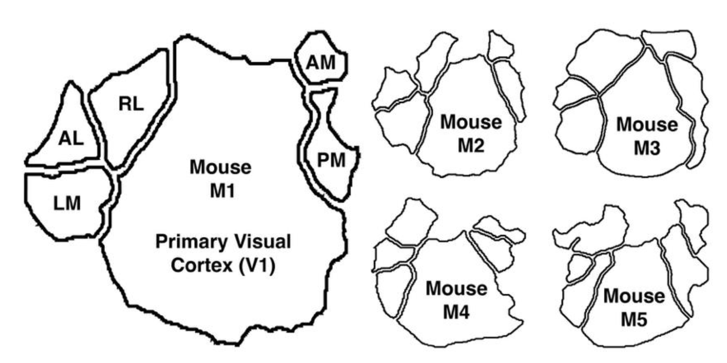
Figure 2.
Mice M1-M5 in the same layout as Figure 1, each showing a single frame of fluorescence intensity for the indicator GCaMP6s. We show a segment of these data evolving in time in Supplementary Movie 1.
Figure 2.
Mice M1-M5 in the same layout as Figure 1, each showing a single frame of fluorescence intensity for the indicator GCaMP6s. We show a segment of these data evolving in time in Supplementary Movie 1.
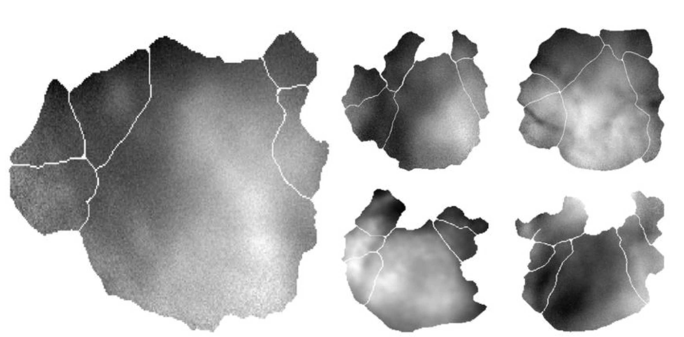
Figure 3.
A)We show a Gaussian distribution evolving according to a diffusion process at an early point in time
Figure 3.
A)We show a Gaussian distribution evolving according to a diffusion process at an early point in time
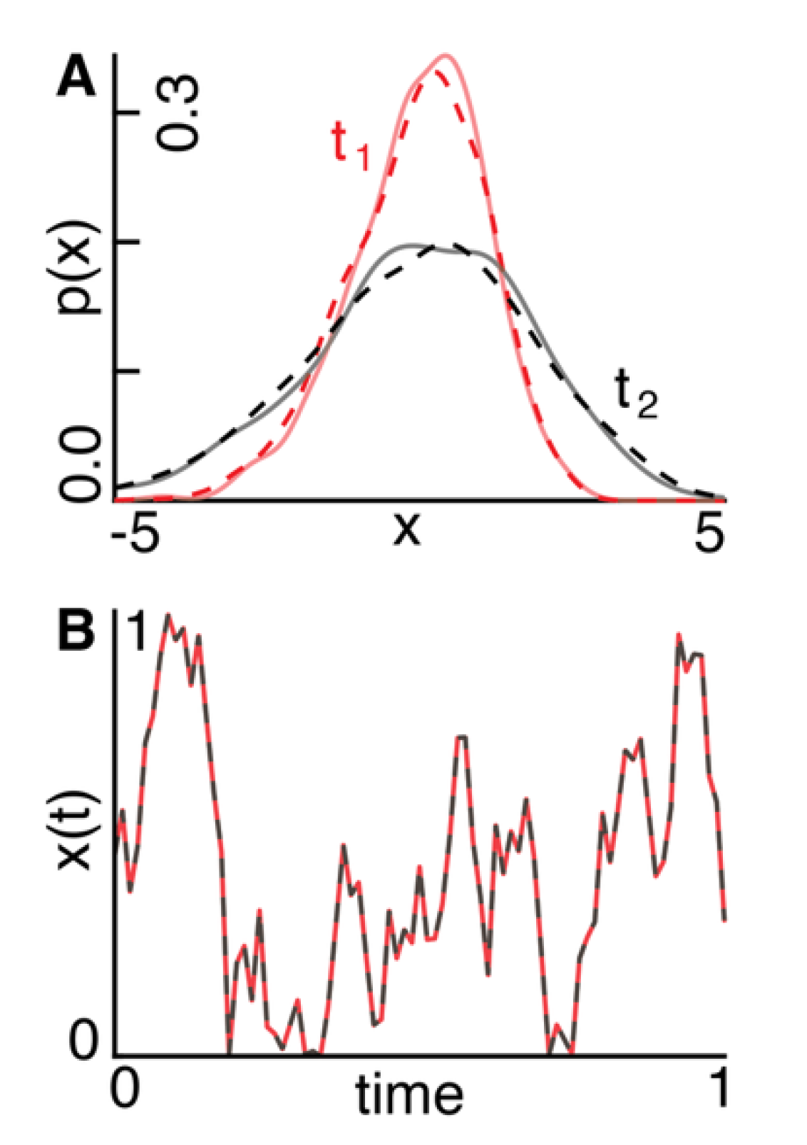
Figure 4.
A segment of the normalized first principal component of two-photon signal amplitude from area AM in mouse M3 is shown in black. The red trace shows the result of using V1 to predict activity in AM with the mixed-flow transformation model.
Figure 4.
A segment of the normalized first principal component of two-photon signal amplitude from area AM in mouse M3 is shown in black. The red trace shows the result of using V1 to predict activity in AM with the mixed-flow transformation model.
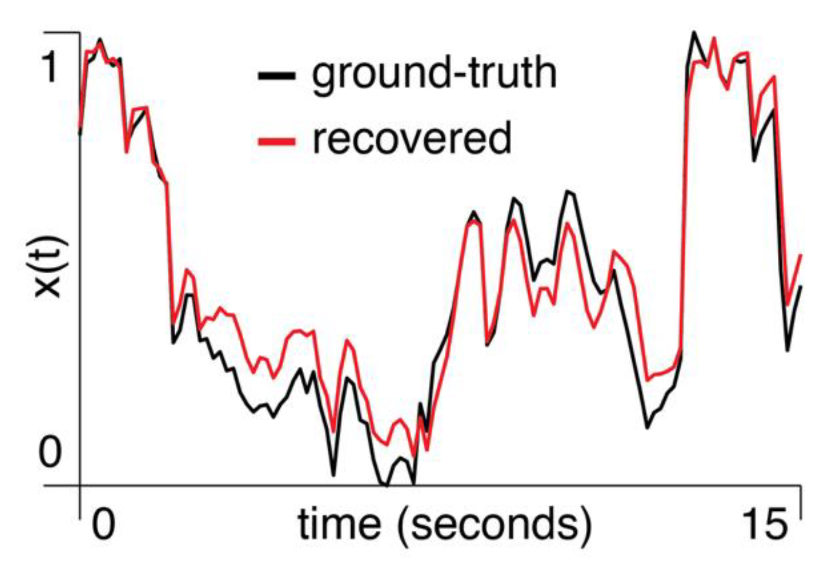
Figure 5.
Pairwise directional predictability between brain regions: anterolateral (A), anteromedial (M), lateromedial (L), posteromedial (P), rostrolateral (R), and primary visual cortex (V). Regional signals were extracted using the first principal component of the voxel time series within each region. Mice M1-M5 from Figure 1 are shown from left-to-right and the grayscale colour bar indicates the coefficient of determination () between region pairs, computed via a directional predictive model. Only connections that survived false discovery rate (FDR) correction and exceeded an are shown.
Disclaimer/Publisher’s Note: The statements, opinions and data contained in all publications are solely those of the individual author(s) and contributor(s) and not of MDPI and/or the editor(s). MDPI and/or the editor(s) disclaim responsibility for any injury to people or property resulting from any ideas, methods, instructions or products referred to in the content. |
© 2025 by the authors. Licensee MDPI, Basel, Switzerland. This article is an open access article distributed under the terms and conditions of the Creative Commons Attribution (CC BY) license (http://creativecommons.org/licenses/by/4.0/).
Copyright: This open access article is published under a Creative Commons CC BY 4.0 license, which permit the free download, distribution, and reuse, provided that the author and preprint are cited in any reuse.


