
Submitted:
26 February 2025
Posted:
26 February 2025
You are already at the latest version
Abstract
The paper presents measured vibration magnitudes on the trough surface and on the frame of a laboratory model of a vibrating conveyor, detected by acceleration sensors. The vibration source is a DC asynchronous vibration motor with two discs with unbalanced masses mechanically attached to the end parts of the rotor. The trough of the vibrating conveyor is supported by four rubber springs of two types, which are characterized by considerable spring stiffness. Digital signals measured by the sensors, which carry information about the magnitude of acting vibrations, can be remotely transmitted from their place of action via a WI-FI router to the operating station, where they are subjected to the deailed computer based analysis. The highest mean magnitude of the effective vibration velocity (4.8 mm·s-1) in the vertical direction was measured on a model vibrating conveyor, with rubber springs of stiffness of 54 N·mm-1, with the unloaded trough without the conveyed material. The lowest mean magnitude of the effective vibration velocity (1.2 mm·s-1) in the vertical direction with a weight of 5.099 kg of conveyed material on the trough. Rubber springs, of optimum stiffness, dampen the vibrations transmitted to the machine frame. From their sizes, it is possible to remotely monitor the working operation of the vibrating conveyor or to obtain information about the failure of one or several used rubber springs. The paper provides guidance on how to design an optimum spring stiffness, which has a major impact on the magnitude of vibrations transmitted to the frame or foundations of a particular vibratory machine design. Measured signals from acceleration sensors detecting the magnitude of the vibration allow remote monitoring of the optimum operating condition of the vibration equipment depending on predetermined parameters, namely the trough inclination angle, the throw angle, the rotor speed of the vibration motor, the spring stiffness and the amount of material on the trough surface.
Keywords:
vibrating conveyor
; harmonic vibration
; effective speed value
; sensor vibration measurement
; circular motion of trough
1. Introduction
In vibrating conveyors or separators the vibration is considered to be the movement of the trough and other structural parts, individual parts of which oscillate around the equilibrium position [1].
The level of vibration of the trough transmitted to the frame or foundation, to which the frame of the vibrating machines [2] is mechanically attached, is significantly influenced by a number of parameters, the most important of which are the weight of the trough not filled with material and the rotor speed of the vibrating motor.
In condition monitoring, vibration measurement can be used to indicate and monitor the operational performance of vibrating conveyors or vibrating sorters. It is the aim of this paper to demonstrate that from the analysis of the measured vibration signals on the frame of the vibrating conveyor using sensors, it is possible to remotely monitor its working activity and obtain information about the mass or volume quantity [3] of the conveyed or sorted material located on the trough.
Vibrations of the trough or frame of the vibrating conveyor [4] are given by means of a combination of six movements - displacement in the orthogonal system of x, y, z coordinates and rotation around these x, y, z axes (such a mechanical system has six degrees of freedom). However, the majority of mechanical systems do not oscillate as a single fixed point; waves are generated instead [5].
Harmonic vibrations are periodic vibrations (i.e., the time course of the vibrodiagnostic quantities is repeated) containing a single frequency. The harmonic vibration is beneficial in that that if we determine at least one of the determining quantities (deflection, velocity or acceleration) then remaining quantities can be calculated according to the relations [6], [7].
In the article [8], P. Czubak and M. Gajowy attempt to identify important elements determining the design of an anti-resonant type conveyor. The article analyses the impacts of various types of suspension and the ratio of the body mass to the mass of the conveyor trough on forces transmitted to the ground are analysed.
M. Sturm in the article [9] presents a dynamic model, based on a two-mass absorber system, helping to avoid the transfer of vibrations to the ground.
In the article [10] G. Cieplok presents a spatial model of a vibrating conveyor supported on steel-elastomer vibration isolators and vibrated by two inertial vibrators is presented in this article. The results of analyses of the effect of the layout of vibrators on the operation of the conveyor are presented.
In the study [11], a new vibrating conveyor designed for precise material dosing was investigated. The transport possibilities in the circum-resonance zone were tested analytically as well as by simulation. The optimal working point of the system, allowing to lower the vibration amplitude of the eliminator on its own suspension, was found.
M. Sturm in the article [12] established a dynamic model for the targeted displacement of the centre of elasticity of a one-mass conveyor, enabling an optimal motion of the conveyor by an optimized set of springs, connecting the conveying element to the frame.
The study [13] by C.Y. Lee et al. proposes an innovative design that uses a composite sinusoidal control signal to drive a linear two-stage piezoelectric vibratory feeder. The dynamic characteristics of this feeder were both investigated by theoretical formulation and experimental measurement. It is found that the conveying performance of this feeder is better suited for using the composite signal with two sinusoidal components of double frequency.
The mathematical model of the single-mass vibratory screening conveyor equipped with the proposed exciter is developed using the Lagrange-d’Alembert principle, see V. Korendiy et al. [14]. The simulation of the system kinematic and dynamic characteristics under different operational conditions is carried out in the Mathematica software using the integrated Runge-Kutta methods.
In general, the motion of bodies in mechanics (including the vibration of vibrating conveyor troughs or vibrating screen surfaces) can be described by the acceleration a(t) [m·s-2], velocity v(t) [m·s-1], displacement y(t) [m], frequency f [Hz] or period T = f−1 [s-−1]. All these variables are mathematically interrelated.
The oscillation rate is used at low and medium frequencies (f = 10 Hz to 1 kHz) to identify disturbances manifested in these frequencies. Consequently, the vibration rate time history is used for the analysis at lower machine revolutions (for higher frequencies f = 1 kHz to 20 kHz the vibration acceleration is used).
In the article [15] W. Zmuda and P. Czubak determined the dependence of the transport speed of the tested conveyor as a function of the excitation frequency. Favorable excitation frequencies at transports in the main and reversal directions were found, and the high usefulness of the machine in the production lines requiring accurate material dosage was indicated.
The amplitude of the harmonic oscillation (A = ymax(t) [m] - maximum deflection) is often replaced by another characteristic to describe the harmonic signal: mean value = 0.637-amplitude of oscillation (yave = 0.637∙A [m]) or rms value (RMS) = 0.707∙amplitude of oscillation (yRMS = 0.707∙A [m] [6]). The effective vibration value yRMS [m] (the so-called root mean square value), replaces the vibration time history y(t) [m] by a constant energy value.
A theoretical analysis of synchronization of inertial vibrators of a vibratory conveyor with adynamic damper is presented in this paper [16]. This paper builds on the findings of papers [14] and [10] and presents a more detailed analysis of synchronization processes in anti-resonant devices. While the paper [14] focuses on asymmetric vibrators and their effect on the dynamic behavior of the device, the paper [16] deepens this approach with an emphasis on optimizing the synchronization of drive vibrators. Compared to the paper [10], which focuses on self-synchronization in conventional vibratory conveyors, this paper highlights unique characteristics of anti-resonance systems.
The paper [17] is about the implementation of a two-stage vibration insuation system for a “Shake-Out” conveyor. Its authors W. Fiebiech and J. Wrobel describe the effect of various insulation levels on reducing the transmission of vibrations to the equipment frame and surrounding structures.
The article [18] presents a method of vibrating screen trajectory control based on MR (magnetorheological) dampers applied in a screen suspension. Authors A. Ogonowski and P. Krauze present a mathematical description of the dynamic screen model was derived, and parameters of this model were estimated based on experimental data from a semi-industrial vibrating screen.
The new type of the reversible, vibratory conveyor in which a smooth velocity control (within the full range) in both directions is possible, is presented in the article [19].
The paper [20] focuses on the issue of vibration insulation of vibrating conveyors and its effect on the reduction of vibration transmission to the structural frame and foundations. The authors analyse various types of vibration insulation elements, such as rubber dampers, spring systems and viscous dampers, and evaluate their effectiveness under various operating conditions. The study encompasses both theoretical analysis and experimental measurements that confirm the effectiveness of various insulation methods. In contrast to the paper [10], which deals with the general effects of physical parameters on vibration insulation, this paper focuses more on specific insulation methods and their practical application. Compared to the paper [17], which describes two-stage vibration insulation, this text provides a more in-depth analysis of various insulation technologies and their effectiveness at various vibration frequencies.
The new type of the reversible, vibratory conveyor in which a smooth velocity control (within the full range) in both directions is possible, is presented in papers [21,22]. The study [21] combines mathematical modelling and laboratory tests to investigate the influence of system parameters on the synchronization effect.
The paper [23] is devoted to the analysis of operational properties of vibratory conveyors, which principle of operations is based on the Frahm’s dynamic elimination effect. In order to investigate the correctness of the machine operation the physical model of the conveyor with a feed [24] was constructed and then its mathematical model was developed. The paper [24] is complementary to paper [20], which deals with vibration insulation, but instead of rubber and air springs, leaf springs are examined.
The paper [25] deals with modelling and experimental verification of the dynamic behaviour of a vibrating conveyor with a controlled centrifugal exciter. The study investigates the effectiveness of vibration transmission and how to optimise its settings. This paper extends the findings of the paper [14] with experimental investigations and adds a more detailed analysis of controlled vibration in material sorting applications.
In the paper [26] P. Czubak and W. Surowka present the design and experimental testing of a self-adjusting vibrating conveyor that automatically adapts to changes in load and operating conditions. The authors analyze its performance characteristics and the possibilities of its deployment in industry. This paper is complementary to [19], which focuses on the controlled change of speed and direction of the conveyors movement. Howerver, in this case, the authors investigate the automatic adaptability of the conveyor to various operating conditions.
2. Materials and Methods
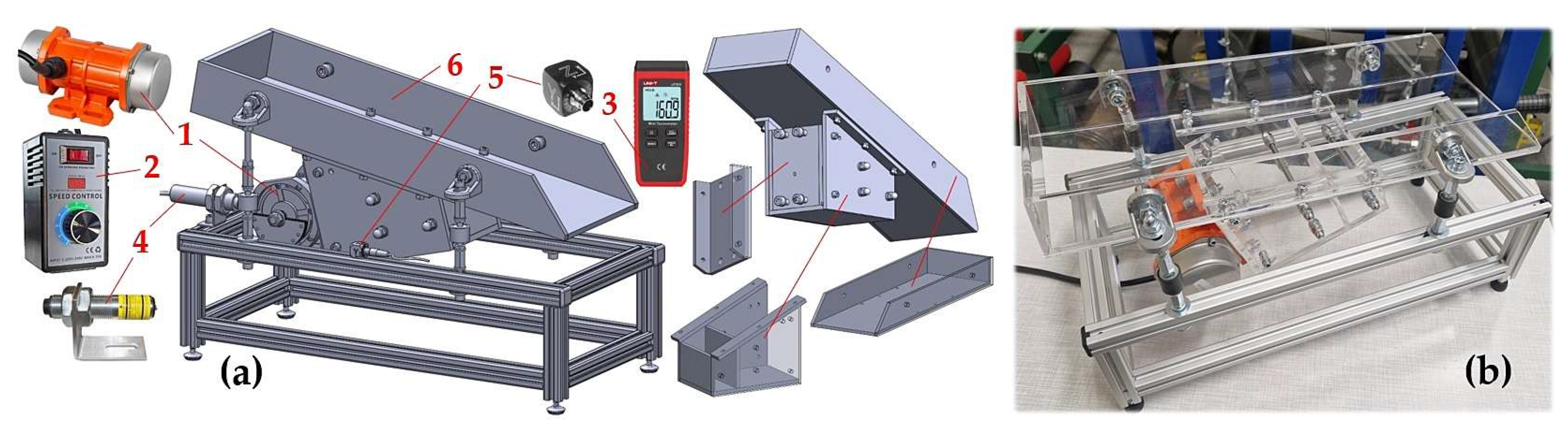
For the design of the experimental device, see Figure 1, has been designed at Department of Machine and Industrial Design, Faculty of Mechanical Engineering, VSB-Technical University of Ostrava, in the software environment of SolidWorks® Premium 2012×64 SP5.0.
The experimental device consists of frame 1 (made of AL profiles of cross-section 20×20 mm, type MI 20×20 I5 [27]), trough 2 (made by “Valter Špalek - Plexi” from Plexiglas 6 mm thick) and supporting elements including rubber springs 3. A vibrating motor 4 [28] (powerPe = 40 W, speed ne = 3000·min-1) is attached to the trough 2, which can be tilted by an angle β = 0 to 15 deg with respect to the horizontal plane, by means of screw connections.
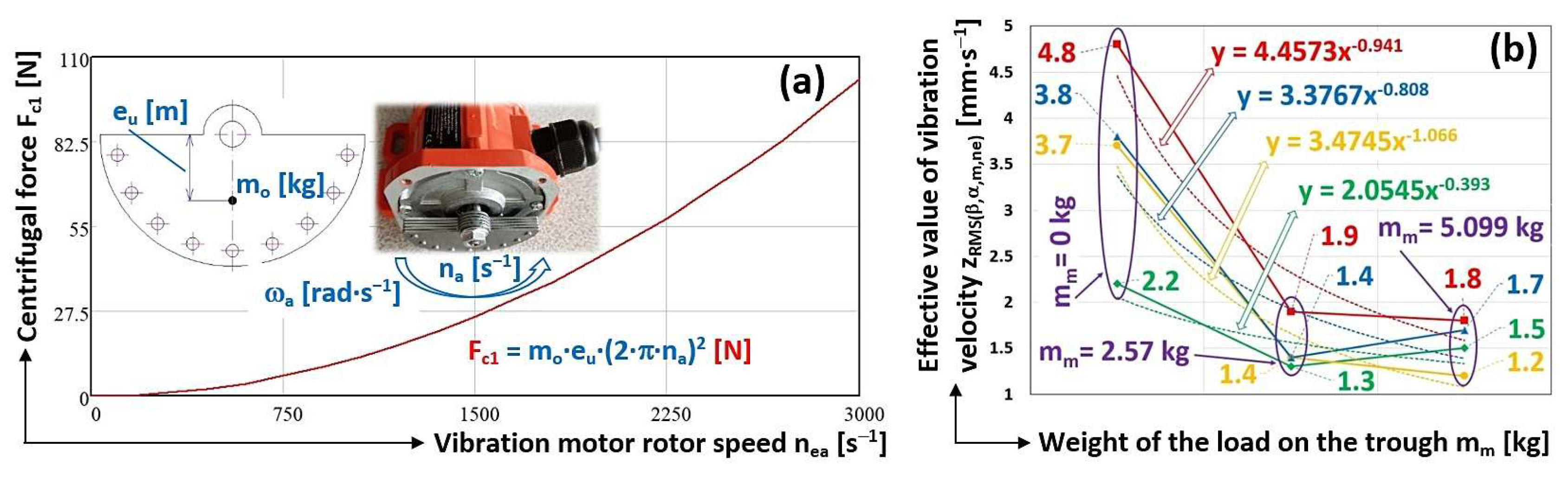
On the rotor shaft of the asynchronous single-phase vibration motor 4 there are two eccentric weights, each with a mass mo [kg] (mo = 80.44·10-3 kg, see 3D model, Figure 2(c), created in SolidWorks® Premium 2012×64 SP5.0 [29]). Eccentricity eu [m], see Figure 2(b), expresses the radius of rotation of the centre of gravity T of the weight.
When the motor rotor rotates at the actual speed nea [s-1], each eccentric weight (see Figure 2(c)) of the vibration motor generates the centrifugal force Fc1 [N] (1), assuming that ωa [rad·s-1] (2) is the instantaneous angular velocity of the rotating weight.
Trough oscillation frequency f [Hz], when using electromagnetic exciters [30] is usually identical to the AC frequency of 50 Hz in Europe (60 Hz in the U.S.), it represents the number of cycles of the T sinusoid per second.
The instantaneous value of the centrifugal force Fc [N] in the axis of oscillation (which is inclined at an angle α = 10° to 25° to the horizontal plane, the so-called throw angle α [deg], see Figure 1(c)) can be quantified according to (1).
The force Fc [N] (1) must keep in a continuous oscillating motion with predetermined oscillation parameters (deflection, frequency f [Hz], angle of throw α [deg]) the mass mt [kg], which is given by the sum of masses of the trough of the vibrating conveyor, the exciter and the material conveyed on the trough.
The trough of the vibrating conveyor 2, to which the vibrating motor 4 is mechanically attached at an angle of α [deg], oscillates with harmonic (periodic) motion. The instantaneous deflection y(t) [m] (3) of the periodically oscillating trough (it takes both positive and negative values) expresses the instantaneous distance of the centre of gravity T of the trough 2 from its equilibrium position.
The diagram expressing the dependence of the instantaneous deflection y(t) [m] on time t [s] is called a time diagram and has the shape of a sinusoid, see Figure 3(a).
A condition for the transport of material by a vibratory conveyor with a microblast is that the highest value of the acceleration a2 [m·s-2] (tj. při ω·t = -1) acting on the material grain, see Figure 3(b), is higher than the gravitational acceleration g [m·s-2].
The angular frequency f [s-1] is defined as the inverse value of the period T, i.e., the frequency (see Figure 3), namely the mean number of revolutions of nea [s-1] per unit time. In case of the uniform motion along a circle, the angular frequency f [s-1] is numerically equal (if the angular velocity is considered as a scalar) to the angular velocity ωa [rad·s-1] (2).
The trough oscillates at a frequency f [Hz] at an angle of α [deg] to the direction of traffic (to the horizontal plane). The bottom of the trough, on which the material to be conveyed rests, is alternately in the upper and lower extreme positions.
Component of oscillation in the direction yx(t) [m], see Figure 4(a), and the component in the direction perpendicular to yy(t) [m] to the direction of material motion is described by equation (4).
The instantaneous deflection y(t) [m] of the harmonic vibration of the trough described by the equation (3), and the components of the vibration (assuming trough inclination angle β = 0 deg) in the direction yx(t) [m] (4) and in the direction perpendicular yy(t) [m] (4) to the direction of material movement, with amplitude eu [m] (eccentricity of unbalance eu = 12.95 mm) is presented in Figure 4(b). If the trough is inclined at an angle β [deg] with respect to the horizontal plane, then the oscillation components can be expressed by equation (5).
The harmonic oscillation of the trough mounted on springs of total stiffness ss [N·mm-1] is caused by the force Fa [N] (6), the magnitude of which is directly proportional to the deflection y(t) [m] and has a direction to the equilibrium position at each moment.
The spring stiffness (constant of proportionality) ss [N·m-1] [31] is defined as the fraction of the force F [N] that elongates/shortens the spring by the value ΔL [m].
The mass of the oscillating system mt [kg] can be determined according to relation (7), where me [kg] is the mass of the vibrating motor (me = 1.372 kg, see [28]); mz [kg] is the mass of the plastic trough (including connecting material) (mz = 1.653 kg, determined by weighing); mm [kg] is the mass of the material on the trough (0 kg; 2.570 kg and 5.099 kg).
The natural frequency of the oscillating system f0 [s-1] determined from the angular velocity ω0 [rad·s-1] of the mass mt [kg] can be expressed according to relation (8).
From the ratio of the working frequency of the oscillating system f [s-1] (2) and the natural frequency of the oscillating system f0 [s-1] (7) it is possible to determine, in which region the vibrating machine will work (z = fa/f0 [-]), if z < 1 - is a subresonant region, z = 0.85÷0.95 - resonant region, z > 1÷5 - supra-resonant region.
When a trough assembly with mass mt = 8.124 kg is placed on 4 rubber springs (lengths in free state L0 = 20 mm, D = 18 mm, ss = 54 N·mm-1 [32]), rubber spring with size ΔL1 = 0.37 mm will be compressed due to the applied weight Gt = mt·g = 79.76 N, see Figure 5. Due to the centrifugal force Fc = 15.15 N (1) generated by the eccentric weights of the vibration motor, at the speed nea = 787 min-1, one spring of ΔL2 = 0.07 mm is compressed. According to [7] the maximum permissible compression of the rubber spring is 5.0 mm, which is greater value than ΔLc = ΔL1 + ΔL2 = 0.44 mm.
The magnitude of the centrifugal force Fc [N] (1) generated by the eccentric weights (hmotnosti mo = 80.44·10-3 kg) of the vibration motor reaches the maximum (Fc(max) = 205.62 N) at a moment when the rotor of the vibration motor is rotating at speed ne = 3000 min-1. The maximum allowable compression of the rubber spring is ΔLc(max) = 1.32 mm, which is less than the maximum allowable compression (5.0 mm) of the rubber spring specified by the manufacturer.
Speed of asynchronous single-phase motor of vibration motor 1, see Figure 6, were controlled by a thyristor electronic voltage regulator 2 typ DJ-SC40 [34].
The actual revolutions of the electric motor 1 nea [min-1] were obtained by measuring the speed sensor UNI-T UT373 3 [35]. The rotor revolutions of the asynchronous single-phase motor were monitored in laboratory measurements by an optical laser sensor DS-TACHO-3 4 [36]. Size of compressing 1 piece of rubber spring by size ΔL2 [m], see Figure 5, directly proportionally affect the revolutions nea [s-1] of the vibration motor. At maximum speed ne = 3000·min-1 of the rotor of the vibration motor the centrifugal speed would be (1) Fc = 205.62 N.
Vibrations generated by rotating (nea [s-1] revolutions) eccentric weights (see Figure 2) of the vibration motor, transmitted to the frame of the vibration conveyor, were detected by two acceleration sensors 5 typ PCE KS903.10 [37].
Figure 6.
Vibrating conveyor (a) control and measuring components, (b) realised model with the plastic trough. 1 - vibration motor, 2 - speed controller, 3 - speed sensor, 4 - laser sensor, 5 - acceleration sensor, 6 - plastic trough.
Figure 6.
Vibrating conveyor (a) control and measuring components, (b) realised model with the plastic trough. 1 - vibration motor, 2 - speed controller, 3 - speed sensor, 4 - laser sensor, 5 - acceleration sensor, 6 - plastic trough.
The signals from the acceleration sensors were recorded during the experimental measurements with the measuring apparatus Dewesoft SIRIUSi-HS 6xACC, 2xACC+ [38], see Figure 7. The records of the measured values were transformed by the measuring apparatus to the effective values of the broadband velocity [mm·s-1] in the range of 10÷1·104 Hz (this frequency range is applied to the ISO 10816-3 [39]). The effective values of the vibration velocity iRMS(α,β,m,ne) [mm·s-1] (where i = x, y, z - spatial orientation of the axes of the coordinate system) of the periodic waveform were displayed on the PS monitor in the environment of the measuring software Dewesoft X [40].
3. Results
Three repeated measurements of the effective vibration velocity iRMS(α,β,m,ne) [mm·s–1] [6], [7] of the plexiglas trough and the support frame of the laboratory equipment were carried out under the same technical conditions for various input parameters, which are namely: trough inclination angle β = 0, 5, 10 and 15 deg; throw angle α = 10 to 25 deg; load mass mm = 0 kg, 2.57 kg and 5.099 kg and actual speed nea [s-1] of the rotor of the vibrating electric motor. The trough of the vibrating conveyor model is supported by four pieces of rubber springs. In chapters 3.1 to 3.4, rubber springs (silent blocks) with a diameter of 18 mm, unloaded length H0 = 20 mm, made of NR - natural rubber with a hardness of 45° Shore, stiffness ss = 54 N·mm-1 are used.
One of the acceleration sensors is attached to the upper surface of the plexiglas trough before measurement, while another acceleration sensor is attached to the horizontal surface of the AL profile of the vibrating conveyor frame. A weight of mass mm [kg] is placed on the trough of the vibrating conveyor, inclined at an angle of β [deg]. The electronic speed controller sets the desired revolutions nea [min-1] of the rotor of the vibration motor. For different input parameters α [deg], β [deg], mm [kg] a nea [min-1], vibrations are sensed and the measured signals are converted to effective vibration rate values iRMS(α,β,m,ne) [mm·s–1], which are entered in the tables below. Since the vibration motor is attached to the trough by bolted connections, the trough’s angle of throw is reduced to α = 25° - β [deg] when the trough is deflected (i.e., when the angle of inclination β [deg] is changed) from the parallel position.
Figure 8 presents a randomly selected record of vibration measurements by acceleration sensors (type PCE KS903.10) attached to the upper surface of the trough (diagram in the upper left part of the figure) and to the frame (diagram in the lower left part of the figure) of the vibrating conveyor model in the DEWESoft X software environment. Records of measured effective velocity values iRMS(α,β,m,ne) [mm·s–1] on Figure 8 (and given in the tables in chapters 3.1 to 3.4) present the measured vibration values in the i = x, y, z coordinate axes (x-axis - blue, y-axis - red, z-axis - green).
In the tables, see chapters 3.1 to 3.8, giving the measured effective vibration velocity values iRMS(α,β,m,ne) [mm·s–1 give the values of iRMS(α,β,m,ne)A [mm·s–1], which is the arithmetic mean of all (n = 3 number of repeated measurements) measured vibration values iRMS(α,β,m,ne) [mm·s–1] a κα,n [mm·s–1], which is the marginal error. tα,n [-] (t5%,3 = 4.3) is the Student coefficient for the risk α [%] (α = 5%) and the confidence coefficient P [%] (P = 95%) [41].
3.1. Trough Inclination Angle β = 0 deg, Throw Angle α = 25 deg, Silentblock 18x20 mm M6x10
Table 1 lists the measured effective vibration velocity values of iRMS(α,β,m,ne) [mm·s–1] sensed on the surface of the plexiglas trough and on the supporting structure of the vibrating conveyor for the input values α = 25 deg, β = 0 deg, mm = 0 kg a nea = 833 min-1.
Figure 9(a, b) presents the measured effective vibration velocity values iRMS(α,β,m,ne) [mm·s–1] detected by the PCE KS903.10 acceleration sensors on the trough surface (unladen with material weight) and on the vibrating conveyor frame, at a vibrating motor rotor revolutions of 13.88 s-1.
Figure 9(c, d) presents the measured effective vibration velocity values iRMS(α,β,m,ne) [mm·s–1] detected by the PCE KS903.10 acceleration sensors on the trough surface (loaded with material of mass mm = 2.57 kg) and on the vibrating conveyor frame, at a vibrating motor rotor revolutions of 13.83 s-1.
Table 2 lists the measured effective vibration velocity values of iRMS(α,β,m,ne) [mm·s–1], in three planes perpendicular to each other, sensed on the surface of the Plexiglas trough and on the frame of the vibrating conveyor for input values α = 25 deg, β = 0 deg, mm = 2.57 kg a nea = 830 min-1.
Table 3 lists the measured effective vibration velocity values of iRMS(α,β,m,ne) [mm·s–1], in three planes perpendicular to each other, sensed on the surface of the Plexiglas trough and on the frame of the vibrating conveyor for input values α = 25 deg, β = 0 deg, mm = 5.099 kg a nea = 839 min-1.
Figure 10(a, b) presents the measured effective vibration velocity values iRMS(α,β,m,ne) [mm·s–1] detected by the PCE KS903.10 acceleration sensors on the trough surface (loaded with material of mass mm = 5.099 kg) and on the vibrating conveyor frame, at a vibrating motor rotor revolutions of 13.98 s-1.
3.2. Trough Inclination Angle β = 5 deg, Throw Angle α = 20 deg, Silentblock 18x20 mm M6x10
Table 4 lists the measured effective vibration velocity values of iRMS(α,β,m,ne) [mm·s–1], in three planes perpendicular to each other, sensed on the surface of the Plexiglas trough and on the frame of the vibrating conveyor for input values α = 20 deg, β = 5 deg, mm = 0 kg a nea = 806 min-1.
Figure 10(c, d) presents the measured effective vibration velocity values iRMS(α,β,m,ne) [mm·s–1] detected by the PCE KS903.10 acceleration sensors on the trough surface (unladen with material weight) and on the vibrating conveyor frame, at a vibrating motor rotor revolutions of 13.43 s-1.
Table 5 lists the measured effective vibration velocity values of iRMS(α,β,m,ne) [mm·s–1], in three planes perpendicular to each other, sensed on the surface of the Plexiglas trough and on the frame of the vibrating conveyor for input values α = 20 deg, β = 5 deg, mm = 2.57 kg a nea = 862 min-1.
Table 6 lists the measured effective vibration velocity values of iRMS(α,β,m,ne) [mm·s–1], in three planes perpendicular to each other, sensed on the surface of the Plexiglas trough and on the frame of the vibrating conveyor for input values α = 20 deg, β = 5 deg, mm = 5.099 kg a nea = 879 min-1.
3.3. Trough Inclination Angle β = 10 deg, Throw Angle α = 15 deg, Silentblock 18x20 mm M6x10
Table 7 lists the measured effective vibration velocity values of iRMS(α,β,m,ne) [mm·s–1], in three planes perpendicular to each other, sensed on the surface of the Plexiglas trough and on the frame of the vibrating conveyor for input values α = 15 deg, β = 10 deg, mm = 0 kg a nea = 816 min-1.
Table 8 lists the measured effective vibration velocity values of iRMS(α,β,m,ne) [mm·s–1], in three planes perpendicular to each other, sensed on the surface of the Plexiglas trough and on the frame of the vibrating conveyor for input values α = 5 deg, β = 10 deg, mm = 2.57 kg a nea = 961 min-1.
Table 9 lists the measured effective vibration velocity values of iRMS(α,β,m,ne) [mm·s–1], in three planes perpendicular to each other, sensed on the surface of the Plexiglas trough and on the frame of the vibrating conveyor for input values α = 15 deg, β = 10 deg, mm = 5.099 kg a nea = 917 min-1.
3.4. Trough Inclination angle β = 15 deg, Throw Angle α = 10 deg, Silentblock 18x20 mm M6x10
Table 10 lists the measured effective vibration velocity values of iRMS(α,β,m,ne) [mm·s–1], in three planes perpendicular to each other, sensed on the surface of the Plexiglas trough and on the frame of the vibrating conveyor for input values α = 10 deg, β = 15 deg, mm = 0 kg a nea = 748 min-1.
Table 11 lists the measured effective vibration velocity values of iRMS(α,β,m,ne) [mm·s–1], in three planes perpendicular to each other, sensed on the surface of the Plexiglas trough and on the frame of the vibrating conveyor for input values α = 10 deg, β = 15 deg, mm = 2.57 kg a nea = 853 min-1.
Figure 11(a, b) presents the measured effective vibration velocity values iRMS(α,β,m,ne) [mm·s–1] detected by the PCE KS903.10 acceleration sensors on the trough surface (loaded with material of mass mm = 2.57 kg) and on the vibrating conveyor frame, at a vibrating motor rotor revolutions of 15.88 s-1.
Figure 11(c, d) presents the measured effective vibration velocity values iRMS(α,β,m,ne) [mm·s–1] detected by the PCE KS903.10 acceleration sensors on the trough surface (loaded with material of mass mm = 5.099 kg) and on the vibrating conveyor frame, at a vibrating motor rotor revolutions of 15.80 s-1.
Table 12 lists the measured effective vibration velocity values of iRMS(α,β,m,ne) [mm·s–1], in three planes perpendicular to each other, sensed on the surface of the Plexiglas trough and on the frame of the vibrating conveyor for input values α = 10 deg, β = 15 deg, mm = 5.099 kg a nea = 948 min-1.
In the above tables, the measured effective vibration velocity values iRMS(α,β,m,ne) [mm·s–1] are affected by the actual magnitude of the centrifugal force Fc1 [N] (1). The size Fc1 [N] determines the actual rotor revolutions nea [s–1] of the vibration motor. Centrifugal force Fc1 [N], see Figure 12(a), increasing exponentially with increasing angular velocity ωa [rad·s–1].
Figure 12(b) gives the mean values of the 3 times measured effective velocity values in the vertical direction (see Table 1 to Table 12), measured on the frame of the vibrating conveyor model. The refracted curves (depicted in colour at Figure 12(b)), which are formed by two lines (passing through three points), are described by the powers of the trend lines (which are the functions that best describe the measured data).
Figure 12.
(a) the magnitude of the centrifugal force induced by the rotating unbalanced mass, (b) the effective values of the vibration velocities in the vertical direction.
Figure 12.
(a) the magnitude of the centrifugal force induced by the rotating unbalanced mass, (b) the effective values of the vibration velocities in the vertical direction.
In order to compare the measured vibration values iRMS(α,β,m,ne) [mm·s−1] (see Table 1 to Table 12, chap. 3.1 to chap. 3.4) measurements were made on the trough surface and on the frame of the vibration machine model, a plastic trough supported on four rubber springs of 18 mm diameter, length in unloaded state of H0 = 20 mm, using rubber springs of 25 mm diameter, length in unloaded state of H0 = 15 mm.
Chapters 3.5 to 3.8 indicate the measured effective vibration velocity values iRMS(α,β,m,ne) [mm·s–1] in three axes perpendicular to each other, for various input parameters, which are namely: trough inclination angle β = 0, 5, 10 and 15 deg; throw angle α = 0 to 25 deg; load massm mm = 0 kg, 2.570 kg and 5.099 kg and actual revolutions nea [s-1] of the rotor of the vibrating electric motor. Rubber springs (silentblocks) with a diameter of 25 mm, unloaded length H0 = 15, stiffness ss = 120 N·mm-1, made of natural rubber with a hardness of 45° Shore were used. The maximum permissible compression of the rubber spring is according to [33] 3.75 mm.
When a trough assembly with mass mt = 8.124 kg is placed on 4 rubber springs (lengths in free state L0 = 15 mm, D = 25 mm, ss = 120 N·mm-1), rubber spring with size ΔL1 = 0.17 mm will be compressed due to the applied weight Gt = mt·g = 79.76 N, see Figure 5. Due to the centrifugal force Fc = 16.51 N (1) generated by the eccentric weights of the vibration motor, at the speed nea = 850 min-1, 1 spring of ΔL2 = 0.03 mm is compressed. According to [33] the maximum permissible compression of the rubber spring is 3.75 mm, which is greater value than ΔLc = ΔL1 + ΔL2 = 0.2 mm. The magnitude of the centrifugal force Fc [N] (1) generated by the eccentric weights (mo = 80.44·10-3 kg) of the vibration motor reaches the maximum (Fc(max) = 205.62 N) at a moment when the rotor of the vibration motor is rotating at speed ne = 3000 min-1. The maximum allowable compression of the rubber spring is ΔLc(max) = 0.59 mm, which is less than the maximum allowable compression (3.75 mm) of the rubber spring specified by the manufacturer.
Not all measured effective vibration velocity values (in three mutually perpendicular x, y, z axes), for three repeated measurements under the same technical conditions, indicated in the tables below in chap. 3.5 (see Table 13) to chap. 3.8, will be presented due to the scope limitations of this paper - not even randomly, selected graphical records of time records of measured effective vibration velocity values (as presented in Figure 13 and Figure 14) by the measuring apparatus Dewesoft SIRIUSi-HS 6xACC, 2xACC+ [38].
3.5. Trough Inclination Angle β = 0 deg, Throw Angle α = 25 deg, Silentblock 25x15 mm M6x12
Three repeated measurements of the effective vibration velocity iRMS(α,β,m,ne) [mm·s–1] [6], [7] of the plexiglas trough and the support frame of the laboratory equipment were carried out under the same technical conditions for various input parameters, which are namely: trough inclination angle β = 0, 5, 10 and 15 deg; throw angle α = 10 to 25 deg; load mass mm = 0 kg, 2.57 kg and 5.099 kg and actual speed nea [s-1] of the rotor of the vibrating electric motor. The trough of the vibrating conveyor model is supported by four pieces of rubber springs. In chapters 3.5 to 3.8, rubber springs (silent blocks) with a diameter of 25 mm, unloaded length H0 = 15 mm, made of NR – natural rubber with a hardness of 45° Shore, stiffness ss = 1834 N·mm-1 [32,33] are used.
Table 13 lists the measured effective vibration velocity values of iRMS(α,β,m,ne) [mm·s–1], in three planes perpendicular to each other, sensed on the surface of the Plexiglas trough and on the frame of the vibrating conveyor for input values α = 25 deg, β = 0 deg, mm = 0 kg a nea = 761 min-1.
Table 14 lists the measured effective vibration velocity values of iRMS(α,β,m,ne) [mm·s–1], in three planes perpendicular to each other, sensed on the surface of the Plexiglas trough and on the frame of the vibrating conveyor for input values α = 25 deg, β = 0 deg, mm = 2.57 kg a nea = 830 min-1.
Table 15 lists the measured effective vibration velocity values of iRMS(α,β,m,ne) [mm·s–1], in three planes perpendicular to each other, sensed on the surface of the Plexiglas trough and on the frame of the vibrating conveyor for input values α = 25 deg, β = 0 deg, mm = 5.099 kg a nea = 750 min-1.
3.6. Trough Inclination Angle β = 5 deg, Throw Angle α = 20 deg, Silentblock 25x15 mm M6x12
Table 16 lists the measured effective vibration velocity values of iRMS(α,β,m,ne) [mm·s–1], in three planes perpendicular to each other, sensed on the surface of the Plexiglas trough and on the frame of the vibrating conveyor for input values α = 20 deg, β = 5 deg, mm = 0 kg a nea = 847 min-1.
Table 17 lists the measured effective vibration velocity values of iRMS(α,β,m,ne) [mm·s–1] sensed on the surface of the plexiglas trough and on the supporting structure of the vibrating conveyor for the input values α = 20 deg, β = 5 deg, mm = 2.57 kg a nea = 828 min-1.
Figure 13(a, b) presents the measured effective vibration velocity values iRMS(α,β,m,ne) [mm·s–1] detected by the PCE KS903.10 acceleration sensors on the trough surface (loaded with material of mass mm = 2.57 kg) and on the vibrating conveyor frame, at a vibrating motor rotor revolutions of 12.08 s-1.
Table 18 lists the measured effective vibration velocity values of iRMS(α,β,m,ne) [mm·s–1], in three planes perpendicular to each other, sensed on the surface of the Plexiglas trough and on the frame of the vibrating conveyor for input values α = 20 deg, β = 5 deg, mm = 5.099 kg a nea = 746 min-1.
Figure 13(c, d) presents the measured effective vibration velocity values iRMS(α,β,m,ne) [mm·s–1] detected by the PCE KS903.10 acceleration sensors on the trough surface (loaded with material of mass mm = 5.099 kg) and on the vibrating conveyor frame, at a vibrating motor rotor revolutions of 12.43 s-1.
3.7. Trough Inclination Angle β = 10 deg, Throw Angle α = 15 deg, Silentblock 25x15 mm M6x12
Table 19 lists the measured effective vibration velocity values of iRMS(α,β,m,ne) [mm·s–1] sensed on the surface of the plexiglas trough and on the supporting structure of the vibrating conveyor for the input values α = 15 deg, β = 10 deg, mm = 0 kg a nea = 817 min-1.
Figure14(a, b) presents the measured effective vibration velocity values iRMS(α,β,m,ne) [mm·s–1] detected by the PCE KS903.10 acceleration sensors on the trough surface (unladen with material weight) and on the vibrating conveyor frame, at a vibrating motor rotor revolutions of 13.62 s-1.
Table 20 lists the measured effective vibration velocity values of iRMS(α,β,m,ne) [mm·s–1], in three planes perpendicular to each other, sensed on the surface of the Plexiglas trough and on the frame of the vibrating conveyor for input values α = 15 deg, β = 10 deg, mm = 2.57 kg a nea = 835 min-1.
Figure 14(c, d) presents the measured effective vibration velocity values iRMS(α,β,m,ne) [mm·s–1] detected by the PCE KS903.10 acceleration sensors on the trough surface (loaded with material of mass mm = 2.57 kg) and on the vibrating conveyor frame, at a vibrating motor rotor revolutions of 13.92 s-1.
Table 21 lists the measured effective vibration velocity values of iRMS(α,β,m,ne) [mm·s–1] sensed on the surface of the plexiglas trough and on the supporting structure of the vibrating conveyor for the input values α = 15 deg, β = 10 deg, mm = 5.099 kg a nea = 779 min-1.
3.8. Trough Inclination Angle β = 15 deg, Throw Angle α = 10 deg, Silentblock 25x15 mm M6x12
Table 22 lists the measured effective vibration velocity values of iRMS(α,β,m,ne) [mm·s–1] sensed on the surface of the plexiglas trough and on the supporting structure of the vibrating conveyor for the input values α = 10 deg, β = 15 deg, mm = 0 kg a nea = 849 min-1.
Table 23 lists the measured effective vibration velocity values of iRMS(α,β,m,ne) [mm·s–1], in three planes perpendicular to each other, sensed on the surface of the Plexiglas trough and on the frame of the vibrating conveyor for input values α = 10 deg, β = 15 deg, mm = 2.57 kg a nea = 751 min-1.
Table 24 lists the measured effective vibration velocity values of iRMS(α,β,m,ne) [mm·s–1] sensed on the surface of the plexiglas trough and on the supporting structure of the vibrating conveyor for the input values α = 10 deg, β = 15 deg, mm = 5.099 kg a nea = 769 min-1.
This section may be divided by subheadings. It should provide a concise and precise description of the experimental results, their interpretation, as well as the experimental conclusions that can be drawn.
4. Discussion
The basic idea behind this paper was to ask whether vibrations measured on the frame of a vibration machine can remotely monitor its working operation and predict its other characteristics.
The aim of the paper has been to demonstrate that it is possible to obtain information about the amount of conveyed material on the trough during the monitored time period from the detected signals measured by vibration acceleration sensors placed on the frame of the vibrating conveyor or sorter. Measured vibration signals detected on the frame of the vibration machine, and processed by the measuring apparatus, allow the machine operator to be informed whether the cylindrical coil springs or rubber springs are in optimum condition or whether they have been damaged or destroyed.
In order to implement any necessary vibration measurements of selected parts of the vibrating machine, it has been necessary to design and construct a model of the vibrating conveyor [32]. Two identical acceleration sensors [37] and one revolution sensor [36] were used to measure the oscillation speed (used at low and medium frequencies f = 10÷1000 Hz). A DC vibration motor was designed as the oscillation source; its revolutions were controlled by a speed controller [34].
A specific solution was the use of rubber springs, so called silentblocks, to absorb kinetic and acoustic vibrations transmitted to the frame of the vibrating conveyor model. In order to evaluate the measurements, and to verify the correctness of the idea of the possibility of using measured signals by acceleration sensors to monitor the operation of the vibration machine, two types of silent blocks were used, differing in their diameter D [m] and their lengths in the unloaded state H0 [m].
The effective values of vibration velocities obtained from the measurements (see Table 1 to Table 24) show agreement with the conclusions presented in [8], where the effects of various types of suspension and the ratio of the weight of the body to the weight of the conveyor trough on the forces transmitted to the floor have been analysed.
Limiting the vibration load on the foundations by optimizing (e.g., hull geometry, weight distribution, and spring stiffness) vibration devices is described in [10]. The conclusions presented in the paper [10] are consistent with the results obtained, from Figure 12(b) it can be seen that the vibrations of the unloaded trough transmitted to the frame of the vibratory conveyor oscillate at a higher value than the trough loaded with the conveyed material.
The results of the measurements of the effective vibration velocity values were realized in this paper for two types of rubber springs, at various trough inclination angle β [deg], throw angle α [deg], i.e., the vector of the excitation force angle Fc [N] with respect to the horizontal plane, and the load mass mm [kg], i.e., the mass of the material located on the trough surface.
The first set of measurements (see chapters 3.1 to 3.4) was carried out for a rubber spring with the diameter D = 18 mm and length H0 = 20 mm, with a stiffness of 54 N·mm-1. In Table 1 and Table 12, the measured (repeated 3 times under the same technical conditions) effective vibration velocity values are recorded. From these measured values, the means and deviations have been calculated according to the Student distribution [41], which are indicated in the last rows of the tables presented in the paper.
The main conclusion from the measurements made can be traced from Figure 12(b). The diagram indicates that with suitably selected spring stiffnesses (for the optimal design of vibratory conveyor spring stiffnesses it is possible to use [42]) supporting the trough of the vibratory conveyor, it is possible to trace from the analysis of vibration signals (transmitted to the machine frame) generated by sensors whether there is a material on the trough [20]. The analysis of Figure 12(b) clearly indicates that the vibration of the unloaded trough (mm = 0 kg) is higher than the vibration of the loaded trough (mm > 0 kg) of the vibrating conveyor, with a suitably chosen stiffness of the rubber springs ss [N·mm-1].
The second set of measurements (see Chapters 3.5 to 3.8) was carried out for a rubber spring with diameter D = 25 mm and length H0 = 15 mm with the stiffness of 120 N·mm-1. In Table 13 to Table 24, the measured effective vibration velocity values are recorded similarly to the previous tables (see Chapters 3.1 to 3.4).
The conclusion drawn from the measurements made (Chapters 3.5 to 3.8) can be traced from Figure 15, which indicates that with inappropriately chosen spring stiffnesses (ss = 120 N·mm-1 v porovnání s optimální tuhostí ss = 54 N·mm-1) supporting the trough of the vibratory conveyor, it can be deduced from the analysis of the vibration signals (transmitted to the machine frame) generated by the sensors that the vibrations of the loaded trough (mm > 0 kg) are higher than the vibrations of the loaded trough (mm = 0 kg) of the vibratory conveyor.
The conclusions reached, supported by measurements of vibrations of an oscillating trough, the oscillation of which is excited by a DC asynchronous vibration motor, correspond to the results presented in [21,22,23].
Our aim has been to verify the vibration values measured by the sensors and the results obtained in this paper and to measure the vibration values (monitored by acceleration sensors) on the frame of the vibrating feeder (i.e., a vibrating conveyor with a short trough length, which is designed for mass dosing of the conveyed bulk material); its amplitude and frequency of trough vibration is generated by an electromagnetic vibration exciter. The frequency of the trough vibration, and thus the effective vibration speed values on the frame of this vibrating feeder, will be controlled by changing the frequency of the power grid vibration (maximum magnitude 50 Hz) by the frequency converter of the required electrical power.
5. Conclusions
In the presented paper, the tables indicate the effective vibration velocity values obtained by measurements, detected by acceleration sensors, on the trough surface and on the frame of the vibrating conveyor model. The trough of the vibrating conveyor, assembled in one unit from three plexiglas parts, is supported by four identical rubber springs of two types, which differ by their stiffness (spring characteristics). The harmonic oscillation of the trough is produced by a DC asynchronous vibrating motor, the actual revolutions of which are controlled by a thyristor electronic speed controller.
The main objective of the realized signal measurements (which define the magnitude of the vibrations in three mutually perpendicular planes) was to determine whether (with varying input values, namely the angle of throw, the angle of inclination of the trough, rotor revolutions of the vibrating motor) it is possible to obtain (from the measured magnitudes of the vibrations acting on the frame of the vibrating conveyor) information about the operating characteristics and the mass of material to be conveyed on the trough with respect to the stiffness of the rubber springs supporting the vibrating masses.
Acceleration magnitudes of the effective vibration velocity values measured by sensors have demonstrated and confirmed that if springs of a particular stiffness supporting the vibrating trough are selected appropriately, it is possible to remotely monitor the correct operational operation of the vibratory conveyor and to have information that the required mass quantity of conveyed/sorted material is on the trough of the vibratory machine.
With the knowledge of the magnitude of the vibrations acting on the frame of a particular vibrating conveyor/sorter (obtained by sensor measurements), with known values of the stiffness of the springs supporting the trough, it is also possible to trace the failure state of their working activities, or to obtain information about the failure or damage of the rubber or steel coil cylindrical springs (used on the vibrating machine).
Signals indicating the magnitude of the vibration values acting on the frame of vibrating conveyors/sorters, transmitted to the control station, allow remote monitoring of the operation of vibrating machines at any time without the need for physical inspection of these devices by authorized persons at a place of their installation.
The obtained data on the magnitudes of the measured signals detected by the vibration sensors allowed to confirm the correctness of the initial idea that (with appropriately designed machine parts) it is possible to monitor the proper working operation and the failure state of vibrating conveyors under operating conditions.
The current trend towards digitalization and computer-controlled or monitored optimum operation of conveyor handling equipment (including vibratory conveyors and vibratory sorters) is made possible by sensors, measuring equipment and digital signal transmission over any distance.
Author Contributions
Conceptualization, L.H.; methodology, L.H.; software, S.P.; validation, L.H. and M.F.; formal analysis, L.H. and S.P.; investigation, L.H.; resources, L.H.; data curation, M.F.; writing—original draft preparation, L.H.; writing—revie and editing, L.H.; visualization, L.H.; supervision, S.P.; project administration, L.H.; funding acquisition, L.H. All authors have read and agreed to the published version of the manuscript.
Funding
This research was funded by “Research and innovation of modern processes and technologies in industrial practice”, grant number SP2025/001” and was funded by MŠMT ČR (Ministry of education youth and sports).
Data Availability Statement
Acknowledgments
In this section, you can acknowledge any support given which is not covered by the author contribution or funding sections. This may include administrative and technical support, or donations in kind (e.g., materials used for experiments).
Conflicts of Interest
The authors declare no conflict of interest. The funders had no role in the design of the study; in the collection, analyses, or interpretation of data; in the writing of the manuscript; or in the decision to publish the results.
References
- Makinde, O.A.; Ramatsetse, B.I., Mpofu, K. Review of vibrating screen development trends: Linking the past and the future in mining machinery industries. Int J Mineral Process. 2015; Volume 145, pp. 17–22. https://www.sciencedirect.com/science/article/pii/S0301751615300417. [CrossRef]
- Jiang, H.; Zhao, Y.; Duan, C.; Xuliang, Y.; Liu, C.; Wu, J., et al. Kinematics of variable-amplitude screen and analysis of particle behavior during the process of coal screening. Powder Technol. 2017; Volume 306, pp. 88–95. https://www.sciencedirect.com/science/article/pii/S0032591016307690. [CrossRef]
- Hrabovsky, L.; Blata, J.; Hrabec, L.; Fries, J. The detection of forces acting on conveyor rollers of a laboratory device simulating the vertical section of a Sandwich Belt Conveyor. Measurement 2023, Volume 207, pp. 112376. [CrossRef]
- Shokhin, A.E.; Krestnikovskii, K.V.; Nikiforov, A.N. On self-synchronization of inertial vibration exciters in a vibroimpact three-mass system. IOP Confer Ser Materials Sci Eng. 2021 Apr; Volume 129(1), pp. 012041. [CrossRef]
- Kreidl, M.; Smid, R. Technická diagnostika: senzory, metody, analýza signálu. Praha: BEN – technická literatura, 2006. Senzory neelektrických veličin. ISBN 80-730-0158-6.
- Hrabovsky, L.; Pravda, S.; Sebesta, R.; Novakova, E.; Kurac, D. Detection of a Rotating Conveyor Roller Casing Vibrations on a Laboratory Machine. Symmetry 2023, Volume 15, pp. 1626. [CrossRef]
- Hrabovsky, L.; Novakova, E.; Pravda, S.; Kurac, D.; Machalek, T. The Reduction of Rotating Conveyor Roller Vibrations via the Use of Plastic Brackets. Machines 2023, Volume 11, pp. 1070. [CrossRef]
- Czubak, P.; Gajowy, M. Influence of selected physical parameters on vibroinsulation of base-exited vibratory conveyors. Open Engineering 2022, Vol. 12(1), pp. 382-393.
- Sturm, M. Two-mass linear vibratory conveyor with reduced vibration transmission to the ground. Vibroengineering PROCEDIA, Vol. 13, pp. 20–23, Sep. 2017, . [CrossRef]
- Cieplok, G. Influence of vibratory conveyor design parameters on the trough motion and the self-synchronization of inertial vibrators. Open Engineering 2024, Vol. 14(1), pp. 20220434. [CrossRef]
- Surowka, W.; Czubak, P. Transport properties of the new vibratory conveyor at operations in the resonance zone. Open Engineering 2021, Vol. 11(1), pp. 1214-1222. [CrossRef]
- Sturm, M. Modification of the motion characteristics of a one-mass linear vibratory conveyor. Vibroengineering PROCEDIA 2018, Vol. 19, pp. 17–21. [CrossRef]
- Lee, C.Y.; Teng, T.A.; Hu, C.-M. A two-way linear piezoelectric vibratory conveyor actuated by a composite sinusoidal voltage input. Journal of Vibroengineering 2021, Vol. 23(2), pp. 316–326. [CrossRef]
- Korendiy, V.; Kuzio, I.; Nikipchuk, S.; Kotsiumbas, O.; Dmyterko, P. On the dynamic behavior of an asymmetric self-regulated planetary-type vibration exciter. Vibroengineering PROCEDIA 2022, Vol. 42, pp. 7–13. [CrossRef]
- Zmuda, W.; Czubak, P. (2022). Investigations of the transport possibilities of a new vibratory conveyor equipped with a single electro-vibrator. Transport Problems 2022, Vol. 17, pp. 127-136. [CrossRef]
- Cieplok, G. (2023). Self-synchronization of drive vibrators of an antiresonance vibratory conveyor. Journal of Theoretical and Applied Mechanics 2023, pp. 501-511. [CrossRef]
- Fiebig, W.; Wrobel, J. Two Stage Vibration Isolation of Vibratory Shake-Out Conveyor. Archives of Civil and Mechanical Engineering 2017, Vol. 17(2), pp. 199-204. https://www.proquest.com/scholarly-journals/two-stage-vibration-isolation-vibratory-shake-out/docview/2932489633/se-2.
- Ogonowski, S.; Krauze, P. (2022). Trajectory Control for Vibrating Screen with Magnetorheological Dampers. Sensors 2022, Vol. 22(11), pp. 4225. [CrossRef]
- Czubak, P. Vibratory conveyor of the controlled transport velocity with the possibility of the reversal operations. Journal of Vibroengineering 2016, Vol. 18(6), pp. 3539–3547. [CrossRef]
- Pesik, M.; Nemecek, P. Vibroisolation of Vibratory Conveyors. Applied Mechanics and Materials 2015, Vol. 732, pp. 253-256. https://www.proquest.com/scholarly-journals/vibroisolation-vibratory-conveyors/docview/1656157399/se-2. [CrossRef]
- Cieplok, G.; Sikora, M. Two-Mass Dynamic Absorber of a Widened Antiresonance Zone. Archive of Mechanical Engineering 2015, Vol. 62(2), pp. 257-277. https://www.proquest.com/scholarly-journals/two-mass-dynamic-absorber-widened-antiresonance/docview/1860849675/se-2.
- Cieplok, G. Wojcik, K. (2020). Conditions for self-synchronization of inertial vibrators of vibratory conveyors in general motion. Journal of Theoretical and Applied Mechanics 2020, Vol. 58, pp. 513-524. [CrossRef]
- Michalczyk, J.; Gajovy, M. Operational Properties of Vibratory Conveyors of the Antiresonance Type. Archives of Mining Sciences 2018; Vol. 63(2). https://journals.pan.pl/dlibra/publication/122449/edition/106728/content.
- Michalczyk, J.; Czubak, P. Latent reactions in suspension systems of vibratory machines supported by leaf springs. Polish Academy of Sciences, Committee on Machine Building 2000; Vol. 47(4). https://journals.pan.pl/dlibra/publication/144147/edition/125384/content.
- Kachur, O.; Korendiy, V.; Lanets, O.; Kachmar, R.; Nazar, I.; Heletiy, V. Dynamics of a vibratory screening conveyor equipped with a controllable centrifugal exciter. Vibroengineering PROCEDIA 2023, Vol. 48, pp. 8–14. [CrossRef]
- Czubak, P. Surowka, W. Transport features of a new, self -attuned conveyor. Transport Problems 2022, Vol. 17, pp. 5-16. [CrossRef]
- AL profil 20x20. Available online: https://www.marek.eu/hlinikove-konstrukcni-profily-mi-system/serie-i/velikost-20-drazka-i5/37483/hlinikovy-profil-20x20-i5.html (accessed on 9 June 2024).
- Vibrating Motor 40W Single Phase. Available online: https://www.vevor.com/ac-vibrator-motor-c_11716/ac-vibration-motor-vibrating-motor-asynchronous-vibrator-40w-110v-single-phase-p_010623131264 (accessed on 16 May 2024).
- SolidWorks Premium 2020. Available online: https://www.freesoftwarefiles.com/graphic-designing/solidworks-premium-2020-free-download/#google_vignette (accessed on 18 Marc 2020).
- Electromagnetic vibration exciter. Available online: https://www.dexinmag.com/productinfo/1224319.html (accessed on 5 January 2025).
- Hrabovsky, L.; Mlcak, T.; Kotajny, G. Forces generated in the parking brake of the pallet locking system. Advances in Science and Technology. Research Journal 2019, Vol. 13(4), pp. 181-187. [CrossRef]
- Hrabovsky, L.; Blata, J.; Kovar, L., Kolesar, M., Stepanik, J. Sensor-Based Detection of Characteristics of Rubber Springs. Journal of Sensor and Actuator Networks 2025; Vol. 14(1). https://www.mdpi.com/2224-2708/14/1/5.
- Silentblocks catalogue. Available online: https://www.elesa-ganter.cz/static/catalogues/files/Silentbloky.pdf (accessed on 15 September 2024).
- AC motor speed controller. Available online: https://www.neven.cz/kategorie/elektronicke-soucastky/stmivace/scr-regulator-otacek/dj-sc40-ac-regulator-napeti-plynuly-2200w/ (accessed on 10 October 2024).
- UNI-T UT373 Handheld LCD Digital Tachometer. Available online: https://www.cafago.com/cs/p-e18774.html (accessed on 2 August 2024).
- DEWESoft General Catalog. Available online: https://d36j349d8rqm96.cloudfront.net/3/6/Dewesoft-DS-NET-Manual-EN.pdf (accessed on 2 May 2021).
- Hand-Arm Acceleration Sensor KS903.10. Available online: https://www.pce-instruments.com/eu/pce-instruments-hand-arm-acceleration-sensor-ks903.10-det_5966162.htm (accessed on 26 September 2021).
- DS-TACHO-3 Technical Reference Manual. Available online: https://downloads.dewesoft.com/manuals/dewesoft-ds-tacho3-manual-en.pdf (accessed on 14 March 2022).
- ČSN ISO 10816-1: Mechanical Vibration—Evaluation of Machine Vibration by Measurements on Non-Rotating Parts—Part 1: General Guidelines (In Czech: Vibrace—Hodnocení Vibrací Strojů na Základě Měření na Nerotujících Částech—Část 1: Všeobecné Směrnice). Czech Office for Standards: Praha, Czech Republic, 1998. Available online: https://www.technicke-normy-csn.cz/csn-iso-10816-1-011412-158753.html (accessed on 17 September 2022).
- DeweSoft X. Available online: https://dewesoft.com/products/dewesoftx (accessed on 11 June 2022).
- Madr, V.; Knejzlik, J.; Kopecny, I.; Novotny, I. Fyzikální Měření (In English: Physical Measurement); SNTL: Prague, Czech Republic, 1991; p. 304, ISBN 80-03-00266-4.
- Mantic, M.; Kulka, J.; Kopas, M.; Faltinova, E.; Hrabovsky, L. Limit states of steel supporting structure for bridge cranes. Zeszyty Naukowe. Transport/Politechnika Śląska 2020, Vol. 108, pp. 141-158. [CrossRef]
- Technical information for rubber silent blocks. Available online: https://www.marek.eu/katalog-obrazku/produkt-25518/60804-technicka-informace-pro-pryzove-silentbloky-cz.pdf?srsltid=AfmBOorfE10BXwcE0fhrkHTcCPJ0trxq5pWw5TBxEsAk3tshqOqvG-Y0 (accessed on 8 December 2024).
Figure 1.
Experimental device created in SolidWorks software (a) 3D model, (b) 2D dimensional sketch. 1 - aluminium frame, 2 - plastic trough, 3 - rubber springs, 4 - vibration motor.
Figure 1.
Experimental device created in SolidWorks software (a) 3D model, (b) 2D dimensional sketch. 1 - aluminium frame, 2 - plastic trough, 3 - rubber springs, 4 - vibration motor.
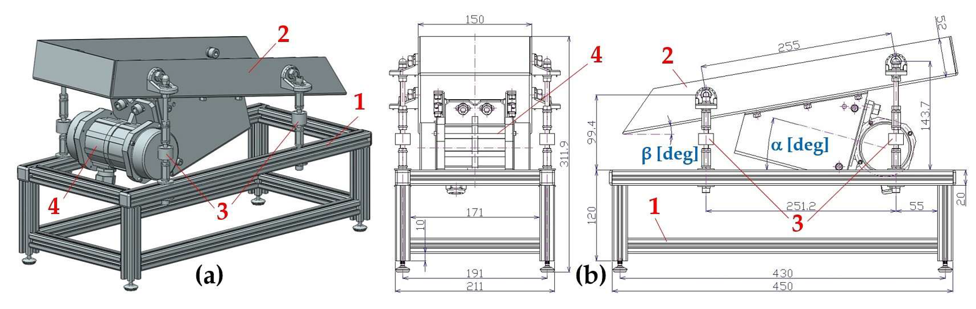
Figure 2.
(a) VEVOR HY-0.4 asynchronous single-phase motor, (b) centre of gravity of the eccentric weight, (c) mass of the eccentric weight.
Figure 2.
(a) VEVOR HY-0.4 asynchronous single-phase motor, (b) centre of gravity of the eccentric weight, (c) mass of the eccentric weight.
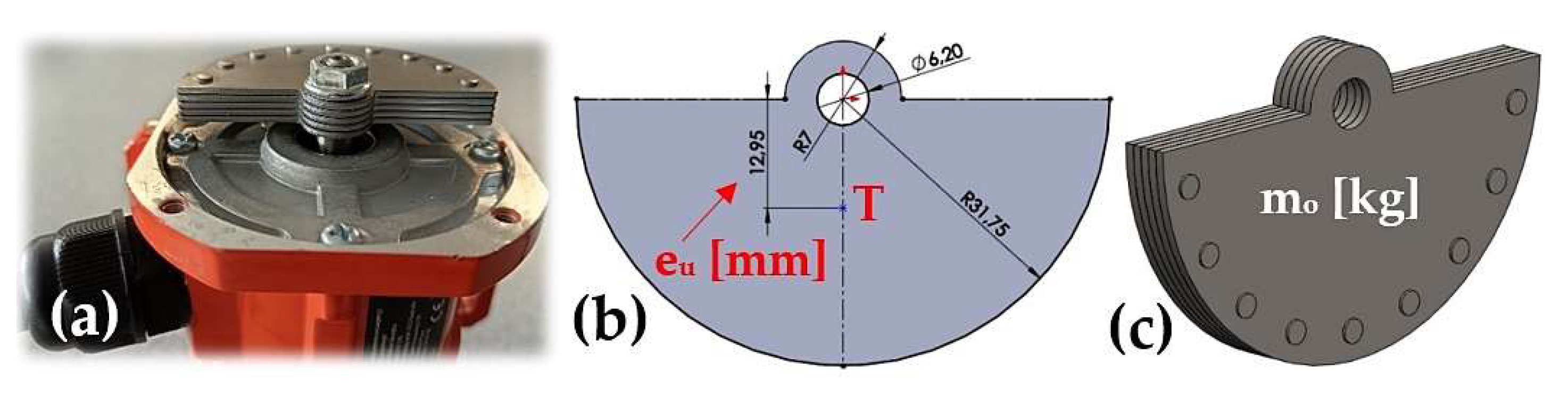
Figure 3.
(a) time diagram of harmonic motion, (b) acceleration ai [m·s-2] of the material grain.
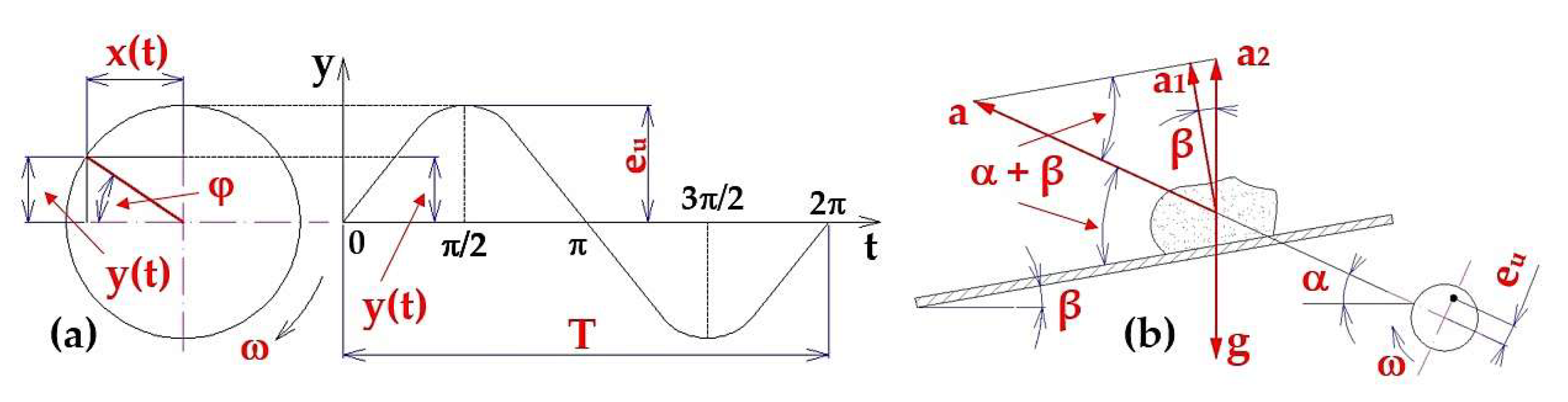
Figure 4.
(a) components of the trough oscillation in the direction yx(t) [m], and in the direction perpendicular yy(t) [m] to the direction of motion, (b) components of the trough oscillation yi(t) [m] at a throw angle α = 20 deg and the eccentricity of unbalance eu = 12.95 mm.
Figure 4.
(a) components of the trough oscillation in the direction yx(t) [m], and in the direction perpendicular yy(t) [m] to the direction of motion, (b) components of the trough oscillation yi(t) [m] at a throw angle α = 20 deg and the eccentricity of unbalance eu = 12.95 mm.
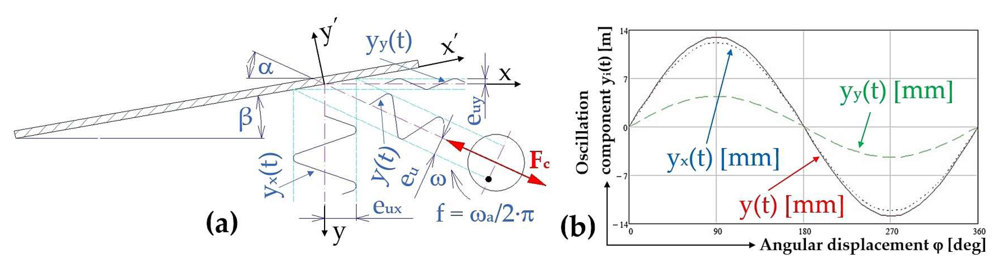
Figure 5.
Elastic deformation of the rubber spring (a) ΔL1 [m] induced by the weight of the system Gs [N], (b) ΔL2 [m] induced by the centrifugal force of the eccentric weights Fc [N], (c) harmonic motion of the system.
Figure 5.
Elastic deformation of the rubber spring (a) ΔL1 [m] induced by the weight of the system Gs [N], (b) ΔL2 [m] induced by the centrifugal force of the eccentric weights Fc [N], (c) harmonic motion of the system.
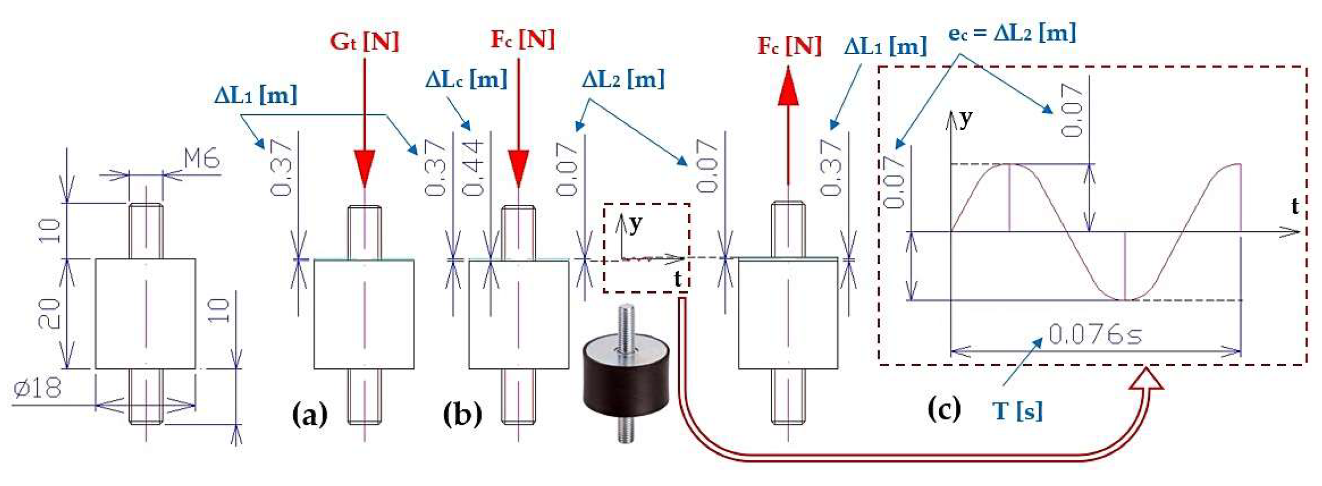
Figure 7.
Measurement chain for detecting and recording vibrations generated by rotating eccentric weights on laboratory equipment.
Figure 7.
Measurement chain for detecting and recording vibrations generated by rotating eccentric weights on laboratory equipment.
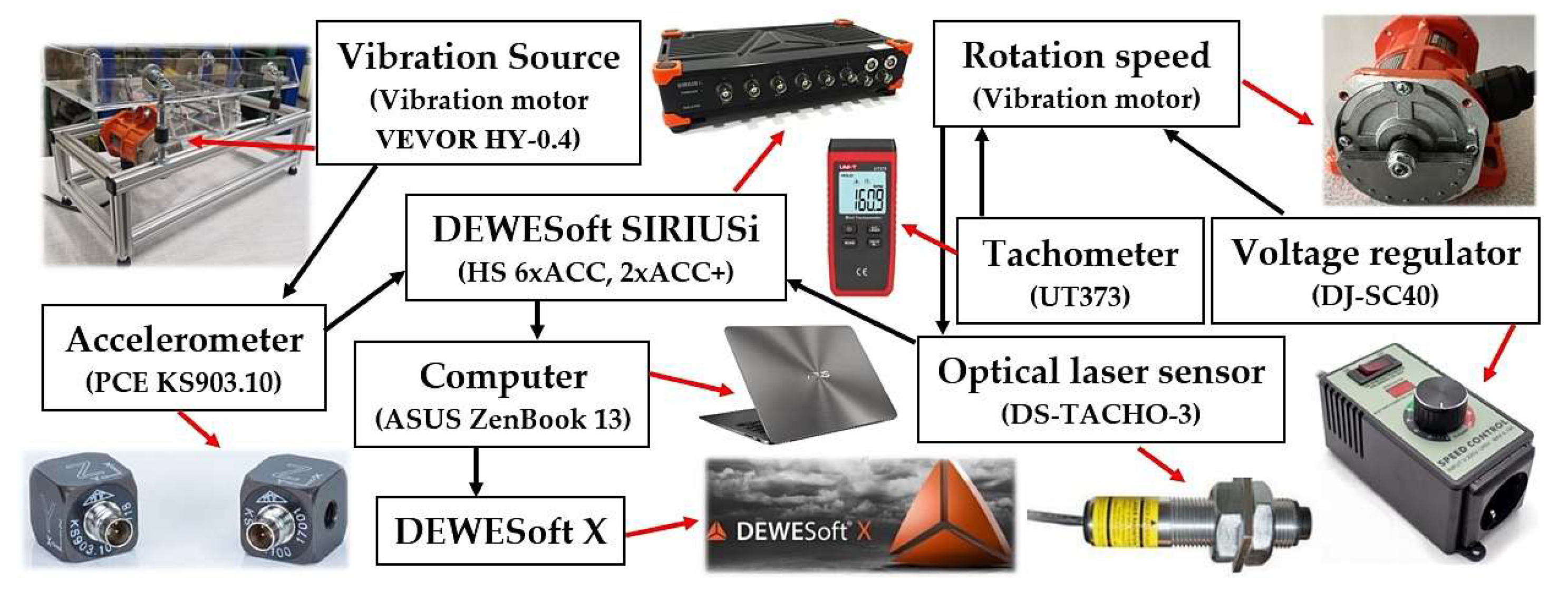
Figure 8.
Records of measured effective vibration velocities by acceleration transducers attached to the trough surface and to the frame of the vibrating conveyor model, in the x-coordinate system (-), y (-), z (-).
Figure 8.
Records of measured effective vibration velocities by acceleration transducers attached to the trough surface and to the frame of the vibrating conveyor model, in the x-coordinate system (-), y (-), z (-).
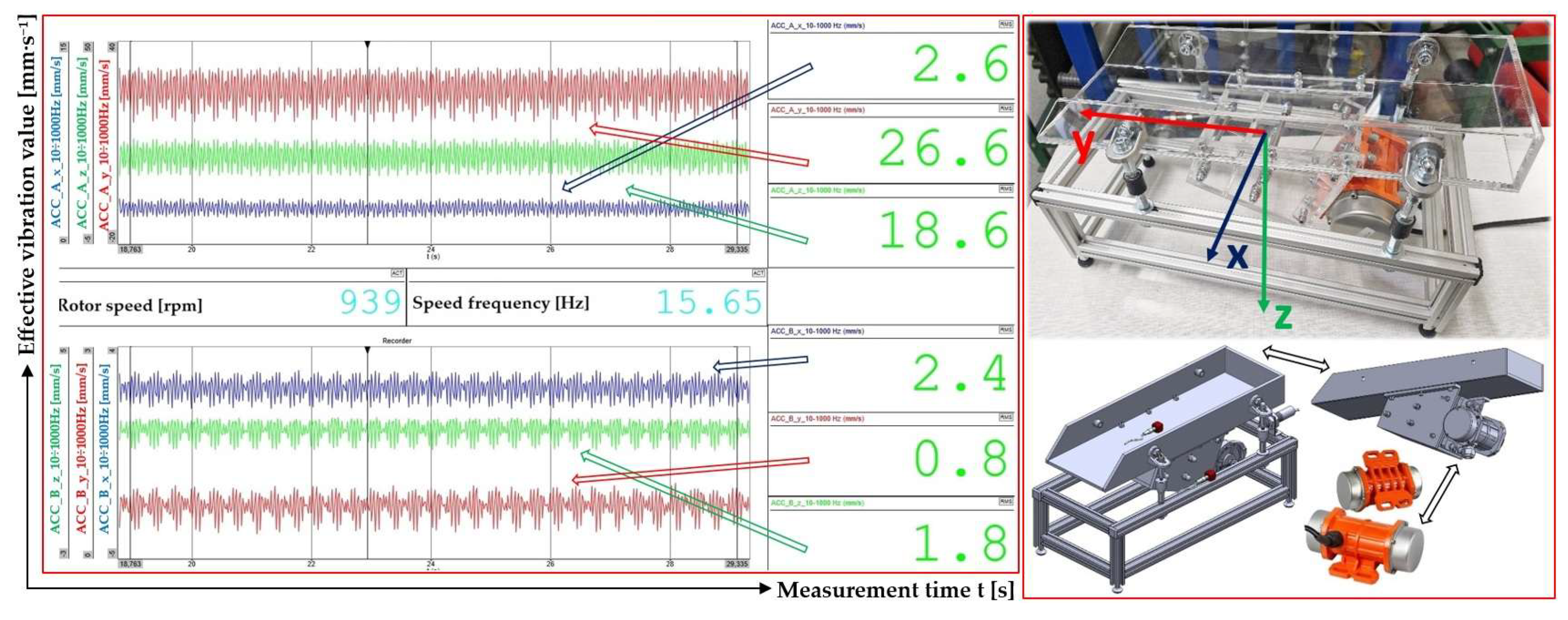
Figure 9.
Effective vibration rate values iRMS(α,β,m,ne) [mm·s–1] measured (a), (c) on the trough surface, (b), (d) on the frame of the vibrating conveyor model.
Figure 9.
Effective vibration rate values iRMS(α,β,m,ne) [mm·s–1] measured (a), (c) on the trough surface, (b), (d) on the frame of the vibrating conveyor model.
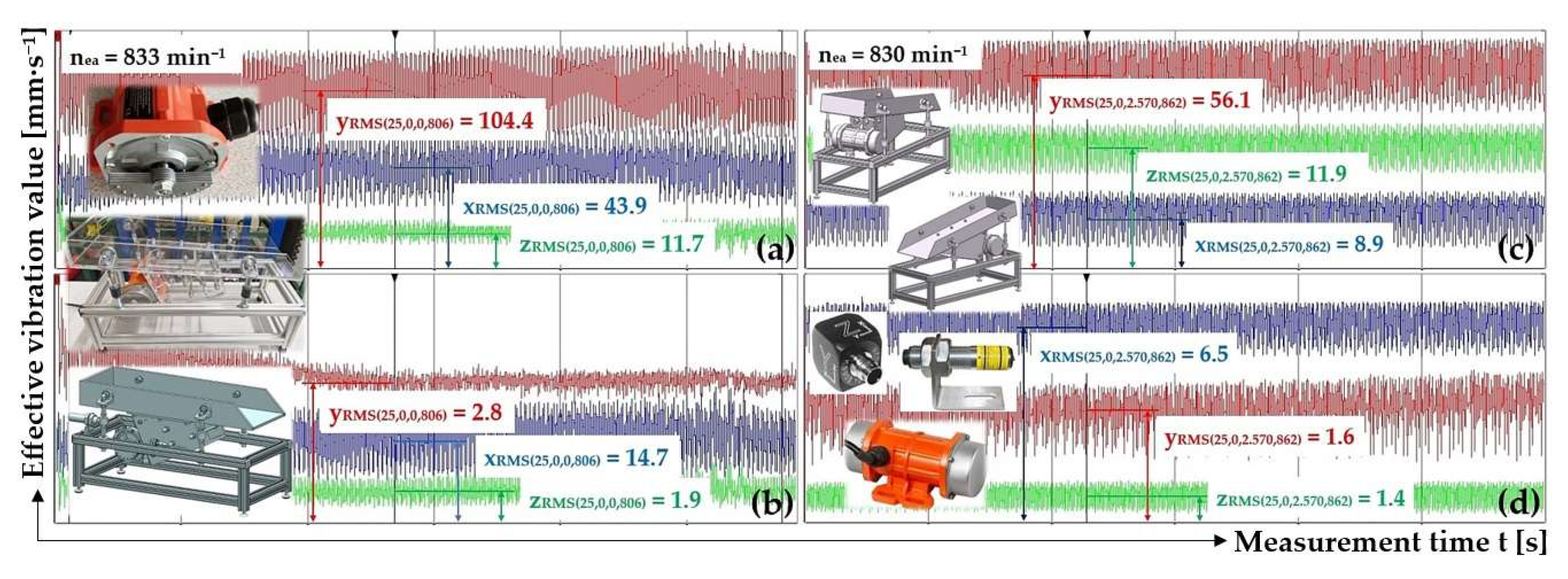
Figure 10.
Effective vibration rate values iRMS(α,β,m,ne) [mm·s–1] measured (a), (c) on the trough surface, (b), (d) on the frame of the vibrating conveyor model.
Figure 10.
Effective vibration rate values iRMS(α,β,m,ne) [mm·s–1] measured (a), (c) on the trough surface, (b), (d) on the frame of the vibrating conveyor model.
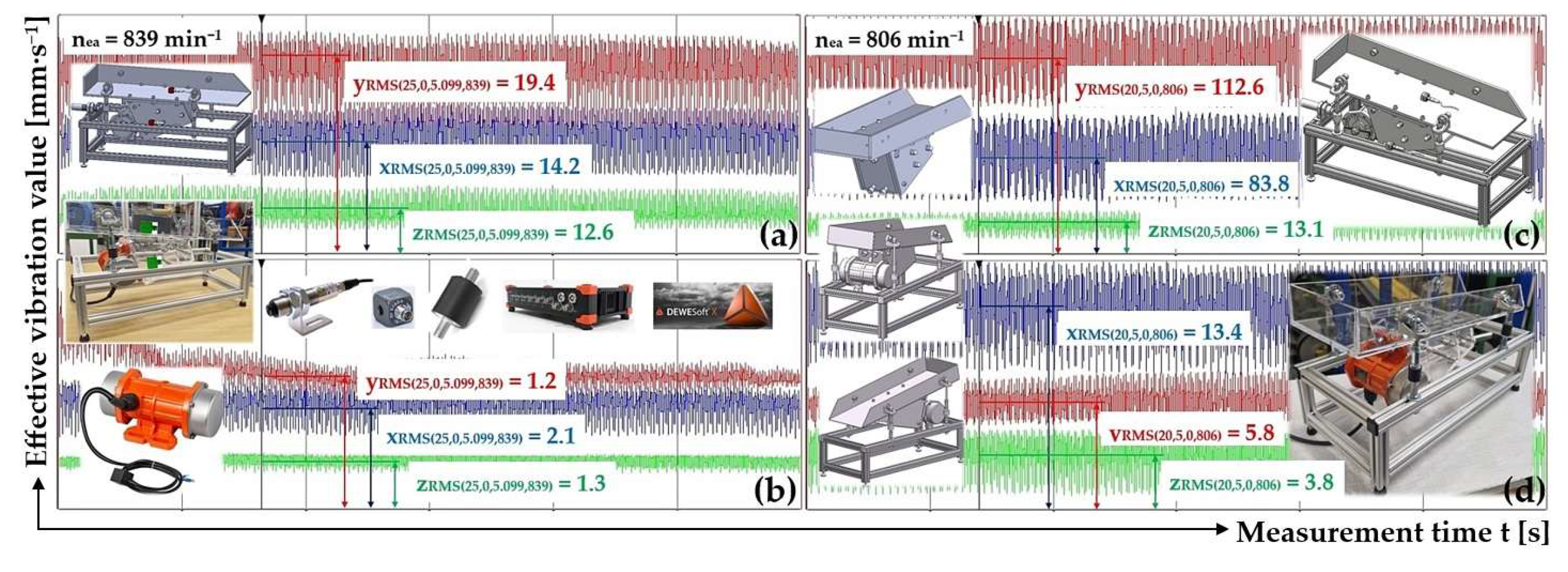
Figure 11.
Effective vibration rate values iRMS(α,β,m,ne) [mm·s–1] measured (a), (c) on the trough surface, (b), (d) on the frame of the vibrating conveyor model.
Figure 11.
Effective vibration rate values iRMS(α,β,m,ne) [mm·s–1] measured (a), (c) on the trough surface, (b), (d) on the frame of the vibrating conveyor model.
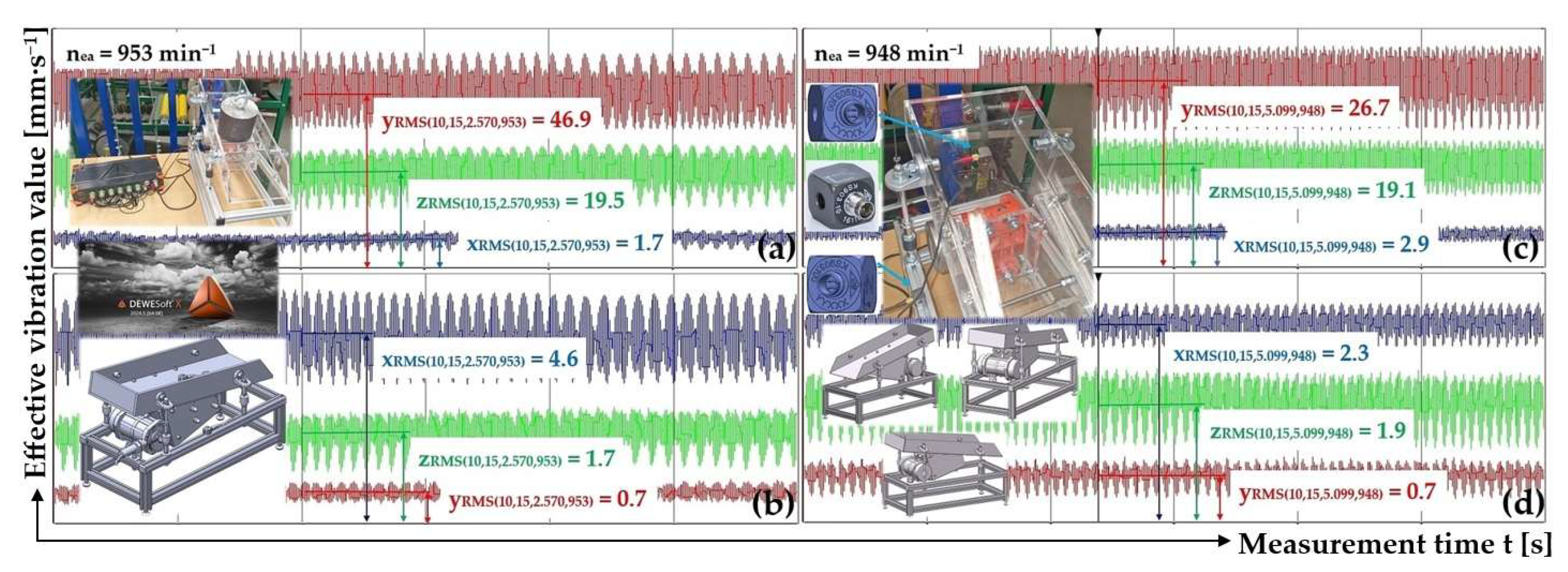
Figure 13.
Effective vibration rate values iRMS(α,β,m,ne) [mm·s–1] measured (a), (c) on the trough surface, (b), (d) on the frame of the vibrating conveyor model.
Figure 13.
Effective vibration rate values iRMS(α,β,m,ne) [mm·s–1] measured (a), (c) on the trough surface, (b), (d) on the frame of the vibrating conveyor model.
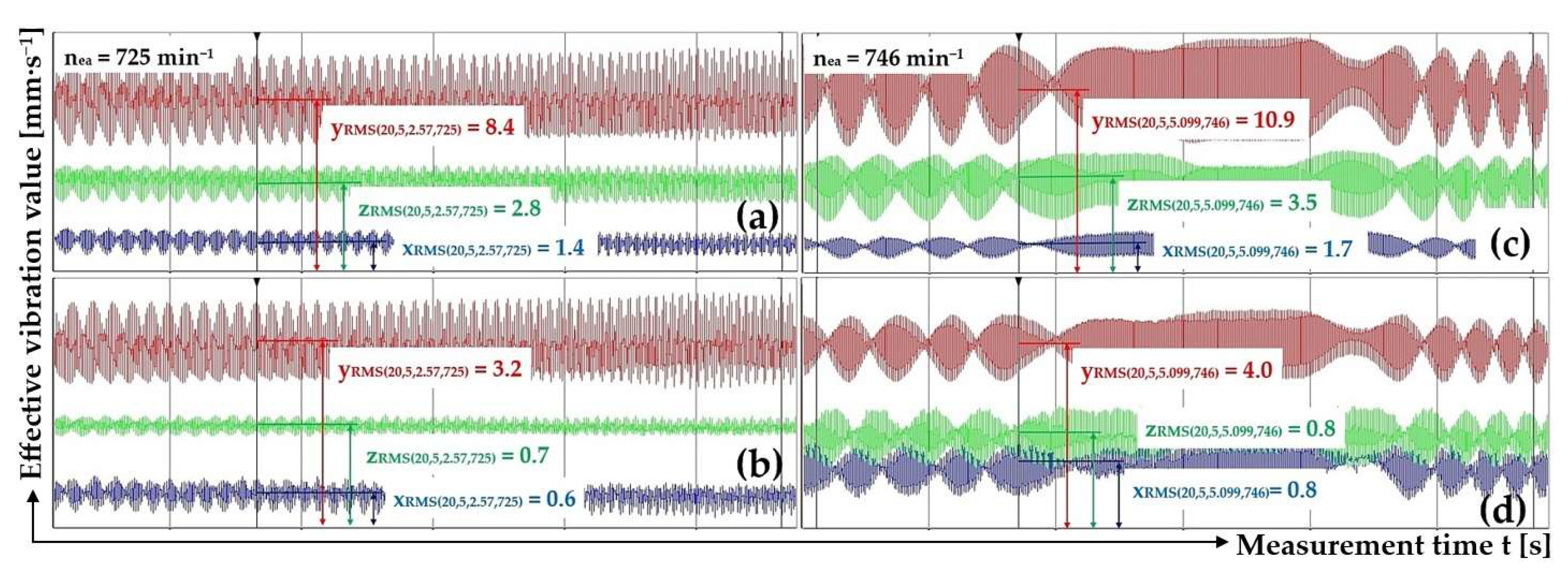
Figure 14.
Effective vibration rate values iRMS(α,β,m,ne) [mm·s–1] measured (a), (c) on the trough surface, (b), (d) on the frame of the vibrating conveyor model.
Figure 14.
Effective vibration rate values iRMS(α,β,m,ne) [mm·s–1] measured (a), (c) on the trough surface, (b), (d) on the frame of the vibrating conveyor model.
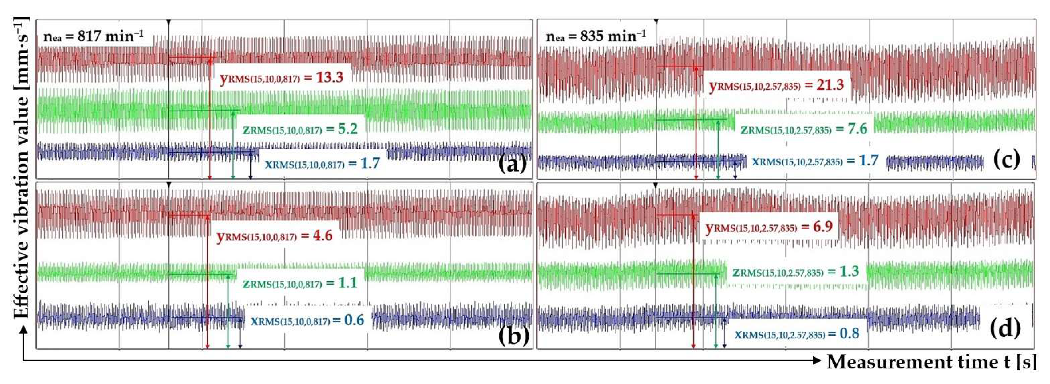
Figure 15.
Effective vibration velocity values zRMS(α,β,m,ne) [mm·s-1] in the vertical direction, monitored on the vibrating conveyor frame.
Figure 15.
Effective vibration velocity values zRMS(α,β,m,ne) [mm·s-1] in the vertical direction, monitored on the vibrating conveyor frame.
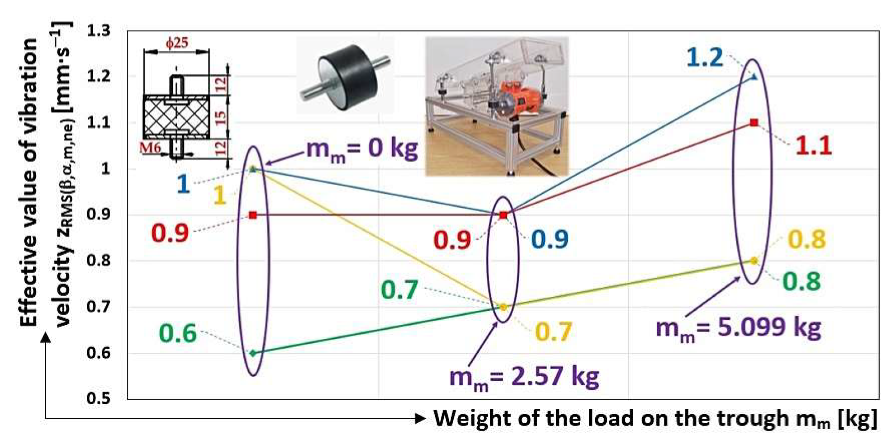

Table 1.
Effective vibration rate values iRMS(α,β,m,ne) [mm·s–1] at mm = 0 kg, nea = 833 min-1.
| nea | β | α | mm | xRMS(α,β,m,ne) | yRMS(α,β,m,ne) | zRMS(α,β,m,ne) | xRMS(α,β,m,ne) | yRMS(α,β,m,ne) | zRMS(α,β,m,ne) |
| s-1 | deg | kg | mm·s–1 | mm·s–1 | |||||
| trough of vibrating conveyor | d frame of vibrating conveyor | ||||||||
| 13.88 | 0 | 25 | 0 | 43.9 1 | 104.4 1 | 11.7 1 | 14.7 2 | 2.8 2 | 1.9 2 |
| 34.3 | 112.2 | 12.3 | 16.0 | 4.4 | 2.5 | ||||
| 38.1 | 108.6 | 11.9 | 15.7 | 3.8 | 2.1 | ||||
| Σ(iRMS(α,β,m,ne)) [mm·s–1] | 116.3 | 325.2 | 35.9 | 46.4 | 11.0 | 6.5 | |||
| iRMS(α,β,m,ne)A ± κ5%,3 [mm·s–1] | 38.8 ± 8.0 | 108.4 ± 6.2 | 12.0 ± 0.5 | 15.5 ± 1.2 | 3.7 ± 1.3 | 2.2 ± 0.5 | |||
Table 2.
Effective vibration rate values iRMS(α,β,m,ne) [mm·s–1] at mm = 2.57 kg, nea = 830 min-1.
| nea | β | α | mm | xRMS(α,β,m,ne) | yRMS(α,β,m,ne) | zRMS(α,β,m,ne) | xRMS(α,β,m,ne) | yRMS(α,β,m,ne) | zRMS(α,β,m,ne) |
| s-1 | deg | kg | mm·s–1 | mm·s–1 | |||||
| trough of vibrating conveyor | frame of vibrating conveyor | ||||||||
| 13.83 | 0 | 25 | 2.57 | 9.8 | 51.4 | 10.4 | 6.1 | 1.4 | 1.2 |
| 8.9 1 | 56.1 1 | 11.9 1 | 6.5 2 | 1.6 2 | 1.4 2 | ||||
| 9.2 | 53.3 | 10.8 | 6.3 | 1.4 | 1.3 | ||||
| Σ(iRMS(α,β,m,ne)) [mm·s–1] | 27.9 | 160.8 | 33.1 | 18.9 | 4.4 | 3.9 | |||
| iRMS(α,β,m,ne)A ± κ5%,3 [mm·s–1] | 9.3 ± 0.8 | 53.6 ± 3.9 | 11.0 ± 1.3 | 6.3 ± 0.3 | 1.5 ± 0.2 | 1.3 ± 0.2 | |||
Table 3.
Effective vibration rate values iRMS(α,β,m,ne) [mm·s–1] at mm = 5.099 kg, nea = 839 min-1.
| nea | β | α | mm | xRMS(α,β,m,ne) | yRMS(α,β,m,ne) | zRMS(α,β,m,ne) | xRMS(α,β,m,ne) | yRMS(α,β,m,ne) | zRMS(α,β,m,ne) |
| s-1 | deg | kg | mm·s–1 | mm·s–1 | |||||
| trough of vibrating conveyor | frame of vibrating conveyor | ||||||||
| 13.98 | 0 | 25 | 5.099 | 13.7 | 24.7 | 15.3 | 2.8 | 1.4 | 1.7 |
| 14.2 1 | 19.4 1 | 12.6 1 | 2.1 2 | 1.2 2 | 1.3 2 | ||||
| 13.9 | 20.6 | 13.4 | 2.6 | 1.4 | 1.5 | ||||
| Σ(iRMS(α,β,m,ne)) [mm·s–1] | 41.8 | 64.7 | 41.3 | 7.5 | 4.0 | 4.5 | |||
| iRMS(α,β,m,ne)A ± κ5%,3 [mm·s–1] | 13.9 ± 0.4 | 21.6 ± 4.9 | 13.8 ± 2.4 | 2.5 ± 0.6 | 1.3 ± 0.2 | 1.5 ± 0.3 | |||
Table 4.
Effective vibration rate values iRMS(α,β,m,ne) [mm·s–1] at mm = 0 kg, nea = 806 min-1.
| nea | β | α | mm | xRMS(α,β,m,ne) | yRMS(α,β,m,ne) | zRMS(α,β,m,ne) | xRMS(α,β,m,ne) | yRMS(α,β,m,ne) | zRMS(α,β,m,ne) |
| s-1 | deg | kg | mm·s–1 | mm·s–1 | |||||
| trough of vibrating conveyor | frame of vibrating conveyor | ||||||||
| 13.43 | 5 | 20 | 0 | 78.7 | 125.5 | 12.8 | 15.9 | 6.9 | 3.6 |
| 83.8 1 | 112.6 1 | 13.1 1 | 13.4 2 | 5.8 2 | 3.8 2 | ||||
| 82.2 | 120.1 | 12.9 | 14.5 | 6.2 | 3.8 | ||||
| Σ(iRMS(α,β,m,ne)) [mm·s–1] | 244.7 | 358.2 | 38.8 | 43.8 | 18.9 | 11.2 | |||
| iRMS(α,β,m,ne)A ± κ5%,3 [mm·s–1] | 81.6 ± 4.4 | 119.4 ± 10.6 | 12.9 ± 0.3 | 14.6 ± 2.0 | 6.3 ± 0.9 | 3.7 ± 0.2 | |||
Table 5.
Effective vibration rate values iRMS(α,β,m,ne) [mm·s–1] at mm = 2.57 kg, nea = 862 min-1.
| nea | β | α | mm | xRMS(α,β,m,ne) | yRMS(α,β,m,ne) | zRMS(α,β,m,ne) | xRMS(α,β,m,ne) | yRMS(α,β,m,ne) | zRMS(α,β,m,ne) |
| s-1 | deg | kg | mm·s–1 | mm·s–1 | |||||
| trough of vibrating conveyor | frame of vibrating conveyor | ||||||||
| 14.37 | 5 | 20 | 2.57 | 21.2 | 58.5 | 16.5 | 6.8 | 2.5 | 1.3 |
| 21.1 | 57.6 | 17.1 | 6.7 | 1.8 | 1.4 | ||||
| 21.2 | 58.1 | 16.9 | 6.8 | 2.2 | 1.4 | ||||
| Σ(iRMS(α,β,m,ne)) [mm·s–1] | 63.5 | 174.2 | 50.5 | 20.3 | 6.5 | 4.1 | |||
| iRMS(α,β,m,ne)A ± κ5%,3 [mm·s–1] | 21.2 ± 0.1 | 58.1 ± 0.7 | 16.8 ± 0.5 | 6.8 ± 0.1 | 2.2 ± 0.6 | 1.4 ± 0.1 | |||
Table 6.
Effective vibration rate values iRMS(α,β,m,ne) [mm·s–1] at mm = 5.099 kg, nea = 879 min-1.
| nea | β | α | mm | xRMS(α,β,m,ne) | yRMS(α,β,m,ne) | zRMS(α,β,m,ne) | xRMS(α,β,m,ne) | yRMS(α,β,m,ne) | zRMS(α,β,m,ne) |
| s-1 | deg | kg | mm·s–1 | mm·s–1 | |||||
| trough of vibrating conveyor | frame of vibrating conveyor | ||||||||
| 14.65 | 5 | 20 | 5.099 | 7.5 | 27.1 | 14.8 | 3.0 | 1.3 | 1.2 |
| 9.3 | 27.0 | 14.2 | 3.0 | 1.6 | 1.2 | ||||
| 8.6 | 27.1 | 14.3 | 3.1 | 1.4 | 1.2 | ||||
| Σ(iRMS(α,β,m,ne)) [mm·s–1] | 25.4 | 81.2 | 43.3 | 9.1 | 4.3 | 3.6 | |||
| iRMS(α,β,m,ne)A ± κ5%,3 [mm·s–1] | 8.5 ± 1.5 | 27.1 ± 0.1 | 14.4 ± 0.6 | 3.0 ± 0.1 | 1.4 ± 0.3 | 1.2 ± 0.0 | |||
Table 7.
Effective vibration rate values iRMS(α,β,m,ne) [mm·s–1] at mm = 0 kg, nea = 816 min-1.
| nea | β | α | mm | xRMS(α,β,m,ne) | yRMS(α,β,m,ne) | zRMS(α,β,m,ne) | xRMS(α,β,m,ne) | yRMS(α,β,m,ne) | zRMS(α,β,m,ne) |
| s-1 | deg | kg | mm·s–1 | mm·s–1 | |||||
| trough of vibrating conveyor | frame of vibrating conveyor | ||||||||
| 13.60 | 10 | 15 | 0 | 3.4 | 88.4 | 20.0 | 17.0 | 2.8 | 3.4 |
| 4.0 | 99.5 | 21.5 | 18.8 | 3.9 | 4.2 | ||||
| 3.9 | 97.1 | 21.3 | 18.2 | 3.2 | 3.8 | ||||
| Σ(iRMS(α,β,m,ne)) [mm·s–1] | 11.3 | 285.0 | 62.8 | 54.0 | 9.9 | 11.4 | |||
| iRMS(α,β,m,ne)A ± κ5%,3 [mm·s–1] | 3.8 ± 0.6 | 95.0 ± 10.2 | 20.9 ± 1.4 | 18.0 ± 1.6 | 3.3 ± 0.9 | 3.8 ± 0.6 | |||
Table 8.
Effective vibration rate values iRMS(α,β,m,ne) [mm·s–1] at mm = 2.57 kg, nea = 961 min-1.
| nea | β | α | mm | xRMS(α,β,m,ne) | yRMS(α,β,m,ne) | zRMS(α,β,m,ne) | xRMS(α,β,m,ne) | yRMS(α,β,m,ne) | zRMS(α,β,m,ne) |
| s-1 | deg | kg | mm·s–1 | mm·s–1 | |||||
| trough of vibrating conveyor | frame of vibrating conveyor | ||||||||
| 16.02 | 10 | 15 | 2.57 | 2.8 | 58.5 | 25.4 | 8.2 | 1.3 | 1.6 |
| 2.4 | 77.3 | 20.5 | 11.0 | 2.0 | 1.3 | ||||
| 2.6 | 77.0 | 23.1 | 9.6 | 1.8 | 1.4 | ||||
| Σ(iRMS(α,β,m,ne)) [mm·s–1] | 7.8 | 212.8 | 69.0 | 28.8 | 5.1 | 4.3 | |||
| iRMS(α,β,m,ne)A ± κ5%,3 [mm·s–1] | 2.6 ± 0.3 | 70.9 ± 19.3 | 23.0 ± 3.9 | 9.6 ± 2.2 | 1.7 ± 0.6 | 1.4 ± 0.3 | |||
Table 9.
Effective vibration rate values iRMS(α,β,m,ne) [mm·s–1] at mm = 5.099 kg, nea = 917 min-1.
| nea | β | α | mm | xRMS(α,β,m,ne) | yRMS(α,β,m,ne) | zRMS(α,β,m,ne) | xRMS(α,β,m,ne) | yRMS(α,β,m,ne) | zRMS(α,β,m,ne) |
| s-1 | deg | kg | mm·s–1 | mm·s–1 | |||||
| trough of vibrating conveyor | frame of vibrating conveyor | ||||||||
| 15.28 | 10 | 15 | 5.099 | 2.3 | 27.9 | 17.3 | 3.5 | 0.8 | 1.5 |
| 3.1 | 27.3 | 19.8 | 3.3 | 0.7 | 1.9 | ||||
| 2.9 | 27.6 | 19.2 | 3.5 | 0.8 | 1.7 | ||||
| Σ(iRMS(α,β,m,ne)) [mm·s–1] | 8.3 | 82.8 | 56.3 | 10.3 | 2.3 | 5.1 | |||
| iRMS(α,β,m,ne)A ± κ5%,3 [mm·s–1] | 2.8 ± 0.7 | 27.6 ± 0.5 | 18.8 ± 2.3 | 3.4 ± 0.2 | 0.8 ± 0.1 | 1.7 ± 0.3 | |||
Table 10.
Effective vibration rate values iRMS(α,β,m,ne) [mm·s–1] at mm = 0 kg, nea = 748 min-1.
| nea | β | α | mm | xRMS(α,β,m,ne) | yRMS(α,β,m,ne) | zRMS(α,β,m,ne) | xRMS(α,β,m,ne) | yRMS(α,β,m,ne) | zRMS(α,β,m,ne) |
| s-1 | deg | kg | mm·s–1 | mm·s–1 | |||||
| trough of vibrating conveyor | frame of vibrating conveyor | ||||||||
| 12.47 | 15 | 10 | 0 | 6.1 | 122.7 | 23.3 | 23.0 | 4.7 | 5.0 |
| 6.1 | 125.7 | 23.6 | 21.3 | 4.1 | 4.7 | ||||
| 6.1 | 124.2 | 23.5 | 21.1 | 4.3 | 4.8 | ||||
| Σ(iRMS(α,β,m,ne)) [mm·s–1] | 18.3 | 372.6 | 70.4 | 65.4 | 13.1 | 14.5 | |||
| iRMS(α,β,m,ne)A ± κ5%,3 [mm·s–1] | 6.1 ± 0.0 | 124.2 ± 2.3 | 23.5 ± 0.3 | 21.8 ± 1.9 | 4.4 ± 0.5 | 4.8 ± 0.3 | |||
Table 11.
Effective vibration rate values iRMS(α,β,m,ne) [mm·s–1] at mm = 2.57 kg, nea = 853 min-1.
| nea | β | α | mm | xRMS(α,β,m,ne) | yRMS(α,β,m,ne) | zRMS(α,β,m,ne) | xRMS(α,β,m,ne) | yRMS(α,β,m,ne) | zRMS(α,β,m,ne) |
| s-1 | deg | kg | mm·s–1 | mm·s–1 | |||||
| trough of vibrating conveyor | frame of vibrating conveyor | ||||||||
| 15.88 | 15 | 10 | 2.57 | 1.7 1 | 46.9 1 | 19.5 1 | 4.6 2 | 0.7 2 | 1.7 2 |
| 1.8 | 44.6 | 21.2 | 4.2 | 0.8 | 2.0 | ||||
| 1.7 | 46.0 | 19.6 | 4.4 | 0.7 | 1.9 | ||||
| Σ(iRMS(α,β,m,ne)) [mm·s–1] | 5.2 | 137.5 | 60.3 | 13.2 | 2.2 | 5.6 | |||
| iRMS(α,β,m,ne)A ± κ5%,3 [mm·s–1] | 1.7 ± 0.1 | 45.8 ± 1.9 | 20.1 ± 1.7 | 4.4 ± 0.3 | 0.7 ± 0.1 | 1.9 ± 0.3 | |||
Table 12.
Effective vibration rate values iRMS(α,β,m,ne) [mm·s–1] at mm = 5.099 kg, nea = 948 min-1.
Table 12.
Effective vibration rate values iRMS(α,β,m,ne) [mm·s–1] at mm = 5.099 kg, nea = 948 min-1.
| nea | β | α | mm | xRMS(α,β,m,ne) | yRMS(α,β,m,ne) | zRMS(α,β,m,ne) | xRMS(α,β,m,ne) | yRMS(α,β,m,ne) | zRMS(α,β,m,ne) |
| s-1 | deg | kg | mm·s–1 | mm·s–1 | |||||
| trough of vibrating conveyor | frame of vibrating conveyor | ||||||||
| 15.80 | 15 | 10 | 5.099 | 2.9 1 | 26.7 1 | 19.1 1 | 2.3 2 | 0.7 2 | 1.9 2 |
| 2.6 | 26.6 | 18.6 | 2.4 | 0.8 | 1.8 | ||||
| 2.7 | 26.6 | 18.9 | 2.4 | 0.8 | 1.8 | ||||
| Σ(iRMS(α,β,m,ne)) [mm·s–1] | 8.2 | 79.9 | 56.6 | 7.1 | 2.3 | 5.5 | |||
| iRMS(α,β,m,ne)A ± κ5%,3 [mm·s–1] | 2.7 ± 0.3 | 26.6 ± 0.1 | 18.9 ± 0.4 | 2.4 ± 0.1 | 0.8 ± 0.1 | 1.8 ± 0.1 | |||
Table 13.
Effective vibration rate values iRMS(α,β,m,ne) [mm·s–1] at mm = 0 kg, nea = 761 min-1.
| nea | β | α | mm | xRMS(α,β,m,ne) | yRMS(α,β,m,ne) | zRMS(α,β,m,ne) | xRMS(α,β,m,ne) | yRMS(α,β,m,ne) | zRMS(α,β,m,ne) |
| s-1 | deg | kg | mm·s–1 | mm·s–1 | |||||
| trough of vibrating conveyor | frame of vibrating conveyor | ||||||||
| 12.68 | 0 | 25 | 0 | 1.4 | 7.3 | 2.4 | 0.8 | 3.3 | 0.6 |
| 1.1 | 6.8 | 2.2 | 0.7 | 3.0 | 0.6 | ||||
| 1.3 | 7.1 | 2.3 | 0.8 | 3.1 | 0.6 | ||||
| Σ(iRMS(α,β,m,ne)) [mm·s–1] | 3.8 | 21.2 | 6.9 | 2.3 | 9.4 | 1.8 | |||
| iRMS(α,β,m,ne)A ± κ5%,3 [mm·s–1] | 1.3 ± 0.3.0 | 7.1 ± 0.4 | 2.3 ± 0.2 | 0.8 ± 0.1 | 3.1 ± 0.3 | 0.6 ± 0.0 | |||
Table 14.
Effective vibration rate values iRMS(α,β,m,ne) [mm·s–1] at mm = 2.57 kg, nea = 830 min-1.
| nea | β | α | mm | xRMS(α,β,m,ne) | yRMS(α,β,m,ne) | zRMS(α,β,m,ne) | xRMS(α,β,m,ne) | yRMS(α,β,m,ne) | zRMS(α,β,m,ne) |
| s-1 | deg | kg | mm·s–1 | mm·s–1 | |||||
| trough of vibrating conveyor | frame of vibrating conveyor | ||||||||
| 12.45 | 0 | 25 | 2.57 | 1.1 | 7.7 | 2.6 | 0.8 | 3.6 | 0.7 |
| 1.1 | 7.6 | 2.4 | 0.8 | 3.4 | 0.7 | ||||
| 1.1 | 7.7 | 2.6 | 0.8 | 3.5 | 0.7 | ||||
| Σ(iRMS(α,β,m,ne)) [mm·s–1] | 3.3 | 23.0 | 7.6 | 2.4 | 10.5 | 2.1 | |||
| iRMS(α,β,m,ne)A ± κ5%,3 [mm·s–1] | 1.1 ± 0.0 | 7.7 ± 0.1 | 2.5 ± 0.2 | 0.8 ± 0.0 | 3.5 ± 0.2 | 0.7 ± 0.0 | |||
Table 15.
Effective vibration rate values iRMS(α,β,m,ne) [mm·s–1] at mm = 5.099 kg, nea = 750 min-1.
Table 15.
Effective vibration rate values iRMS(α,β,m,ne) [mm·s–1] at mm = 5.099 kg, nea = 750 min-1.
| nea | β | α | mm | xRMS(α,β,m,ne) | yRMS(α,β,m,ne) | zRMS(α,β,m,ne) | xRMS(α,β,m,ne) | yRMS(α,β,m,ne) | zRMS(α,β,m,ne) |
| s-1 | deg | kg | mm·s–1 | mm·s–1 | |||||
| trough of vibrating conveyor | frame of vibrating conveyor | ||||||||
| 13.98 | 0 | 25 | 5.099 | 1.2 | 8.7 | 2.5 | 0.8 | 3.8 | 0.8 |
| 1.4 | 9.9 | 2.6 | 0.9 | 4.4 | 0.7 | ||||
| 1.4 | 9.4 | 2.6 | 0.9 | 4.1 | 0.8 | ||||
| Σ(iRMS(α,β,m,ne)) [mm·s–1] | 4.0 | 28.0 | 7.7 | 2.6 | 12.3 | 2.3 | |||
| iRMS(α,β,m,ne)A ± κ5%,3 [mm·s–1] | 1.3 ± 0.2 | 9.3 ± 1.0 | 2.6 ± 0.1 | 0.9 ± 0.1 | 4.1 ± 0.5 | 0.8 ± 0.1 | |||
Table 16.
Effective vibration rate values iRMS(α,β,m,ne) [mm·s–1] at mm = 0 kg, nea = 847 min-1.
| nea | β | α | mm | xRMS(α,β,m,ne) | yRMS(α,β,m,ne) | zRMS(α,β,m,ne) | xRMS(α,β,m,ne) | yRMS(α,β,m,ne) | zRMS(α,β,m,ne) |
| s-1 | deg | kg | mm·s–1 | mm·s–1 | |||||
| trough of vibrating conveyor | frame of vibrating conveyor | ||||||||
| 14.12 | 5 | 20 | 0 | 1.4 | 10.7 | 3.8 | 0.6 | 4.8 | 0.9 |
| 1.6 | 12.7 | 4.0 | 0.7 | 5.3 | 1.1 | ||||
| 1.6 | 12.3 | 3.8 | 0.7 | 5.1 | 1.1 | ||||
| Σ(iRMS(α,β,m,ne)) [mm·s–1] | 4.6 | 35.7 | 11.6 | 2.0 | 15.2 | 3.1 | |||
| iRMS(α,β,m,ne)A ± κ5%,3 [mm·s–1] | 1.5. ± 0.2 | 11.9 ± 1.9 | 3.9 ± 0.2 | 0.7 ± 0.1 | 5.1 ± 0.4 | 1.0 ± 0.2 | |||
Table 17.
Effective vibration rate values iRMS(α,β,m,ne) [mm·s–1] at mm = 2.57 kg, nea = 828 min-1.
| nea | β | α | mm | xRMS(α,β,m,ne) | yRMS(α,β,m,ne) | zRMS(α,β,m,ne) | xRMS(α,β,m,ne) | yRMS(α,β,m,ne) | zRMS(α,β,m,ne) |
| s-1 | deg | kg | mm·s–1 | mm·s–1 | |||||
| trough of vibrating conveyor | frame of vibrating conveyor | ||||||||
| 12.08 | 5 | 20 | 2.57 | 1.4 1 | 8.4 1 | 2.8 1 | 0.6 2 | 3.2 2 | 0.7 2 |
| 1.7 | 9.3 | 3.0 | 0.7 | 3.6 | 0.8 | ||||
| 1.5 | 9.2 | 3.3 | 0.7 | 3.8 | 0.7 | ||||
| Σ(iRMS(α,β,m,ne)) [mm·s–1] | 4.6 | 26.9 | 9.1 | 2.0 | 10.6 | 2.2 | |||
| iRMS(α,β,m,ne)A ± κ5%,3 [mm·s–1] | 1.5 ± 0.3 | 9.0 ± 0.9 | 3.0 ± 0.4 | 0.7 ± 0.1 | 3.5 ± 0.5 | 0.7 ± 0.1 | |||
Table 18.
Effective vibration rate values iRMS(α,β,m,ne) [mm·s–1] at mm = 5.099 kg, nea = 746 min-1.
Table 18.
Effective vibration rate values iRMS(α,β,m,ne) [mm·s–1] at mm = 5.099 kg, nea = 746 min-1.
| nea | β | α | mm | xRMS(α,β,m,ne) | yRMS(α,β,m,ne) | zRMS(α,β,m,ne) | xRMS(α,β,m,ne) | yRMS(α,β,m,ne) | zRMS(α,β,m,ne) |
| s-1 | deg | kg | mm·s–1 | mm·s–1 | |||||
| trough of vibrating conveyor | frame of vibrating conveyor | ||||||||
| 12.43 | 5 | 20 | 5.099 | 1.7 | 9.3 | 3.0 | 0.7 | 3.6 | 0.8 |
| 1.7 1 | 10.9 1 | 3.5 1 | 0.8 2 | 4.0 2 | 0.8 2 | ||||
| 1.8 | 9.9 | 3.1 | 0.8 | 3.3 | 0.8 | ||||
| Σ(iRMS(α,β,m,ne)) [mm·s–1] | 5.2 | 20.1 | 9.6 | 2.3 | 10.9 | 2.4 | |||
| iRMS(α,β,m,ne)A ± κ5%,3 [mm·s–1] | 1.7 ± 0.1 | 10.0 ± 1.3 | 3.2 ± 0.5 | 0.8 ± 0.1 | 3.6 ± 0.6 | 0.8 ± 0.0 | |||
Table 19.
Effective vibration rate values iRMS(α,β,m,ne) [mm·s–1] at mm = 0 kg, nea = 817 min-1.
| nea | β | α | mm | xRMS(α,β,m,ne) | yRMS(α,β,m,ne) | zRMS(α,β,m,ne) | xRMS(α,β,m,ne) | yRMS(α,β,m,ne) | zRMS(α,β,m,ne) |
| s-1 | deg | kg | mm·s–1 | mm·s–1 | |||||
| trough of vibrating conveyor | frame of vibrating conveyor | ||||||||
| 13.62 | 10 | 15 | 0 | 1.7 1 | 13.3 1 | 5.2 1 | 0.6 2 | 4.6 2 | 1.1 2 |
| 1.7 | 12.3 | 4.3 | 0.6 | 4.6 | 0.8 | ||||
| 1.8 | 12.6 | 4.8 | 0.6 | 4.7 | 1.0 | ||||
| Σ(iRMS(α,β,m,ne)) [mm·s–1] | 5.2 | 38.2 | 14.3 | 1.8 | 13.9 | 2.9 | |||
| iRMS(α,β,m,ne)A ± κ5%,3 [mm·s–1] | 1.7 ± 0.1 | 12.7 ± 0.9 | 4.8 ± 0.7 | 0.6 ± 0.0 | 4.6 ± 0.1 | 1.0 ± 0.3 | |||
Table 20.
Effective vibration rate values iRMS(α,β,m,ne) [mm·s–1] at mm = 2.57 kg, nea = 835 min-1.
| nea | β | α | mm | xRMS(α,β,m,ne) | yRMS(α,β,m,ne) | zRMS(α,β,m,ne) | xRMS(α,β,m,ne) | yRMS(α,β,m,ne) | zRMS(α,β,m,ne) |
| s-1 | deg | kg | mm·s–1 | mm·s–1 | |||||
| trough of vibrating conveyor | frame of vibrating conveyor | ||||||||
| 13.92 | 10 | 15 | 2.57 | 1.7 1 | 21.3 1 | 7.6 1 | 0.8 2 | 6.9 2 | 1.3 2 |
| 2.0 | 22.1 | 7.5 | 0.7 | 7.3 | 1.1 | ||||
| 1.8 | 21.6 | 7.5 | 0.8 | 7.1 | 1.3 | ||||
| Σ(iRMS(α,β,m,ne)) [mm·s–1] | 5.5 | 65.0 | 22.6 | 2.3 | 21.3 | 3.7 | |||
| iRMS(α,β,m,ne)A ± κ5%,3 [mm·s–1] | 1.8 ± 0.3 | 21.7 ± 0.7 | 7.5 ± 0.1 | 0.8 ± 0.1 | 7.1 ± 0.3 | 1.2 ± 0.2 | |||
Table 21.
Effective vibration rate values iRMS(α,β,m,ne) [mm·s–1] at mm = 5.099 kg, nea = 779 min-1.
Table 21.
Effective vibration rate values iRMS(α,β,m,ne) [mm·s–1] at mm = 5.099 kg, nea = 779 min-1.
| nea | β | α | mm | xRMS(α,β,m,ne) | yRMS(α,β,m,ne) | zRMS(α,β,m,ne) | xRMS(α,β,m,ne) | yRMS(α,β,m,ne) | zRMS(α,β,m,ne) |
| s-1 | deg | kg | mm·s–1 | mm·s–1 | |||||
| trough of vibrating conveyor | frame of vibrating conveyor | ||||||||
| 12.98 | 10 | 15 | 5.099 | 1.2 | 25.7 | 9.5 | 0.8 | 8.3 | 1.2 |
| 1.0 | 23.6 | 8.3 | 0.7 | 7.6 | 1.1 | ||||
| 1.0 | 26.5 | 9.5 | 0.9 | 8.5 | 1.2 | ||||
| Σ(iRMS(α,β,m,ne)) [mm·s–1] | 3.2 | 75.8 | 27.3 | 2.4 | 24.4 | 3.5 | |||
| iRMS(α,β,m,ne)A ± κ5%,3 [mm·s–1] | 1.1 ± 0.2 | 25.3 ± 2.6 | 9.1 ± 1.2 | 0.8 ± 0.2 | 8.1 ± 0.8 | 1.2 ± 0.1 | |||
Table 22.
Effective vibration rate values iRMS(α,β,m,ne) [mm·s–1] at mm = 0 kg, nea = 849 min-1.
| nea | β | α | mm | xRMS(α,β,m,ne) | yRMS(α,β,m,ne) | zRMS(α,β,m,ne) | xRMS(α,β,m,ne) | yRMS(α,β,m,ne) | zRMS(α,β,m,ne) |
| s-1 | deg | kg | mm·s–1 | mm·s–1 | |||||
| trough of vibrating conveyor | frame of vibrating conveyor | ||||||||
| 14.15 | 15 | 10 | 0 | 2.4 | 15.8 | 6.4 | 0.8 | 5.9 | 1.3 |
| 2.0 | 10.6 | 4.3 | 0.7 | 4.4 | 0.8 | ||||
| 1.6 | 9.8 | 3.8 | 0.6 | 3.9 | 0.7 | ||||
| Σ(iRMS(α,β,m,ne)) [mm·s–1] | 6.0 | 36.2 | 14.5 | 2.1 | 14.2 | 2.8 | |||
| iRMS(α,β,m,ne)A ± κ5%,3 [mm·s–1] | 2.0 ± 0.6 | 12.1 ± 5.8 | 4.8 ± 2.4 | 0.7 ± 0.2 | 4.7 ± 1.8 | 0.9 ± 0.6 | |||
Table 23.
Effective vibration rate values iRMS(α,β,m,ne) [mm·s–1] at mm = 2.57 kg, nea = 751 min-1.
| nea | β | α | mm | xRMS(α,β,m,ne) | yRMS(α,β,m,ne) | zRMS(α,β,m,ne) | xRMS(α,β,m,ne) | yRMS(α,β,m,ne) | zRMS(α,β,m,ne) |
| s-1 | deg | kg | mm·s–1 | mm·s–1 | |||||
| trough of vibrating conveyor | frame of vibrating conveyor | ||||||||
| 12.52 | 15 | 10 | 2.57 | 2.4 | 15.2 | 5.9 | 0.6 | 5.3 | 0.9 |
| 2.8 | 11.9 | 4.9 | 0.5 | 4.3 | 0.7 | ||||
| 3.2 | 11.5 | 5.1 | 0.6 | 4.2 | 0.8 | ||||
| Σ(iRMS(α,β,m,ne)) [mm·s–1] | 8.4 | 38.6 | 15.9 | 1.7 | 13.8 | 2.4 | |||
| iRMS(α,β,m,ne)A ± κ5%,3 [mm·s–1] | 2.8 ± 0.6 | 12.9 ± 3.6 | 5.3 ± 0.9 | 0.6 ± 0.1 | 4.6 ± 1.1 | 0.8 ± 0.2 | |||
Table 24.
Effective vibration rate values iRMS(α,β,m,ne) [mm·s–1] at mm = 5.099 kg, nea = 769 min-1.
Table 24.
Effective vibration rate values iRMS(α,β,m,ne) [mm·s–1] at mm = 5.099 kg, nea = 769 min-1.
| nea | β | α | mm | xRMS(α,β,m,ne) | yRMS(α,β,m,ne) | zRMS(α,β,m,ne) | xRMS(α,β,m,ne) | yRMS(α,β,m,ne) | zRMS(α,β,m,ne) |
| s-1 | deg | kg | mm·s–1 | mm·s–1 | |||||
| trough of vibrating conveyor | frame of vibrating conveyor | ||||||||
| 12.82 | 15 | 10 | 5.099 | 3.1 | 23.8 | 9.8 | 0.3 | 8.4 | 1.1 |
| 3.2 | 24.4 | 10.1 | 0.4 | 8.5 | 1.1 | ||||
| 3.0 | 23.6 | 9.6 | 0.4 | 8.2 | 1.2 | ||||
| Σ(iRMS(α,β,m,ne)) [mm·s–1] | 9.3 | 71.8 | 29.5 | 1.1 | 25.1 | 3.4 | |||
| iRMS(α,β,m,ne)A ± κ5%,3 [mm·s–1] | 3.1 ± 0.2 | 23.9 ± 0.7 | 9.8 ± 0.4 | 0.4 ± 0.1 | 8.4 ± 0.3 | 1.1 ± 0.1 | |||
Disclaimer/Publisher’s Note: The statements, opinions and data contained in all publications are solely those of the individual author(s) and contributor(s) and not of MDPI and/or the editor(s). MDPI and/or the editor(s) disclaim responsibility for any injury to people or property resulting from any ideas, methods, instructions or products referred to in the content. |
© 2025 by the authors. Licensee MDPI, Basel, Switzerland. This article is an open access article distributed under the terms and conditions of the Creative Commons Attribution (CC BY) license (http://creativecommons.org/licenses/by/4.0/).
Copyright: This open access article is published under a Creative Commons CC BY 4.0 license, which permit the free download, distribution, and reuse, provided that the author and preprint are cited in any reuse.


