Nonlinear Anti-Swing Control for Shipboard Cranes with Asymmetric Output Constraints

1. Introduction

Shipboard cranes play a critical role in marine engineering and are widely used for the construction and maintenance of offshore facilities [1], offshore resupply operations [2], and the loading and unloading of cargo on ships [3]. However, due to the complex dynamic characteristics of the system and harsh working conditions at sea, manual operation suffers from low efficiency and poor control precision. This fact has led to an urgent demand for the automated control of shipboard cranes, driving significant advancements in the field. Crane systems are typical underactuated multi-input and multi-output systems with fewer control inputs than the number of outputs. They exhibit highly nonlinear and strongly coupled characteristics, posing considerable challenges to the design of automatic control methods [4,5]. Although substantial progress has been made in controlling land-based cranes [6,7,8,9,10,11,12,13,14], these methods cannot be directly or effectively applied to shipboard cranes. The added complexity of ship motion significantly increases the system's dynamic complexity and internal coupling. Furthermore, the persistent disturbances caused by ocean waves and currents adversely affect the precise transportation of payloads and the suppression of swing.

In recent decades, shipboard cranes have become a research hotspot in the control field and have yielded many significant achievements [15]. The control methods explored in these studies can be broadly categorized into sliding mode control (SMC) [16,17,18], energy-based control [19,20,21], fuzzy logic [22,23], neural network control [24,25], and optimization-based control [26,27], among others. For instance, Kim and Hong [18] proposed a novel adaptive sliding mode control algorithm based on the system model, demonstrating satisfactory disturbance rejection performance. Similarly, Lu et al. [19] developed a nonlinear energy-based controller for shipboard boom cranes, which accounted for both ship roll and heave motions. Unfortunately, existing studies rarely consider or effectively address the issue of output constraints, leaving a critical gap in developing advanced control strategies for shipboard boom cranes.

In practice, the limited workspace or stringent operational requirements often impose constraints on both actuated and unactuated output variables of crane systems, ensuring they remain within appropriate ranges [28]. For instance, the rope length must always remain positive and constrained within a specific range to prevent collisions during transportation. Furthermore, given the instability of the ship’s base and the relatively narrow workspace, it is crucial to ensure precise payload positioning while restricting payload swings within a safe range to avoid accidents. On the other hand, limiting payload swings can effectively enhance system efficiency and reduce energy consumption. To address output constraints in underactuated systems, Li et al. [29] and Lu et al. [30] investigated the constraints on actuated variables. However, their studies neglected the more complex issue of constraints on unactuated states. Although Qian et al. [31] considered constraints on unactuated states, the designed controller theoretically only limited the payload swing angle within a conservative bounded range of (−π/2,π/2). Subsequently, Wang et al. [32] achieved constraints on both actuated and unactuated states within symmetric preset ranges. In order to meet the higher practical requirements of shipboard cranes for transporting payloads, it is necessary to propose a suitable control method to ensure that the output states comply with reasonable preset constraints under harsh environments.

Based on the above discussion, in this paper, considering the actual restricted motion scenario of shipboard cranes, we propose a nonlinear anti-swing control method based on BLFs. The main merits are summarized as follows:

• Stabilizing the ship and the payload is difficult due to unexpected disturbances such as continuous waves. To this end, this paper conducts controller design and theoretical analysis based on the original complex nonlinear dynamics to ensure more reliable performance.
• This method achieves asymmetric motion constraints for the boom luffing angle and rope length by appropriately modifying conventional symmetric barrier functions, ensuring the validity of the rope length under the same sign constraints. For the swing constraints of the unactuated payload, unlike traditional approaches, the proposed method introduces an auxiliary signal to embed the relevant constraint terms into the controller, supported by rigorous theoretical analysis through proof by using reduction to absurdity. Consequently, in contrast to most existing crane-related studies [14,15,16,17,18,19,20,21,22,23,24], which assume the swing angle is confined within a conservative range of (-π/2, π/2), the proposed method removes this assumption. Instead, it flexibly constrains the swing angle within a reasonable range according to practical requirements, making it more adaptable and effective for cargo loading, unloading, and transportation tasks.
• Moreover, the proposed auxiliary signal ingeniously integrates information such as boom luffing velocity and payload swing angle-related information, demonstrating superior swing suppression capabilities compared to existing methods. Theoretical analysis and simulation results validate its effectiveness in accurate positioning and limited swing amplitudes of the payload, which is of significant importance for the challenging operational environments of shipboard cranes.

The remainder of this paper is organized as follows: The "Problem Statement" section explicitly presents the dynamic equations for the shipboard boom crane, its model transformation procedure, and the primary control objectives. Next, the "Controller Design and Stability Analysis" section introduces the main results, including the development of the controller and the closed-loop stability analysis. Subsequently, the "Simulation Results" section includes numerical simulation results and some corresponding analysis to validate the practical performance of the proposed control scheme. Finally, the "Conclusion" section provides some concluding remarks.

2. Problem Statement

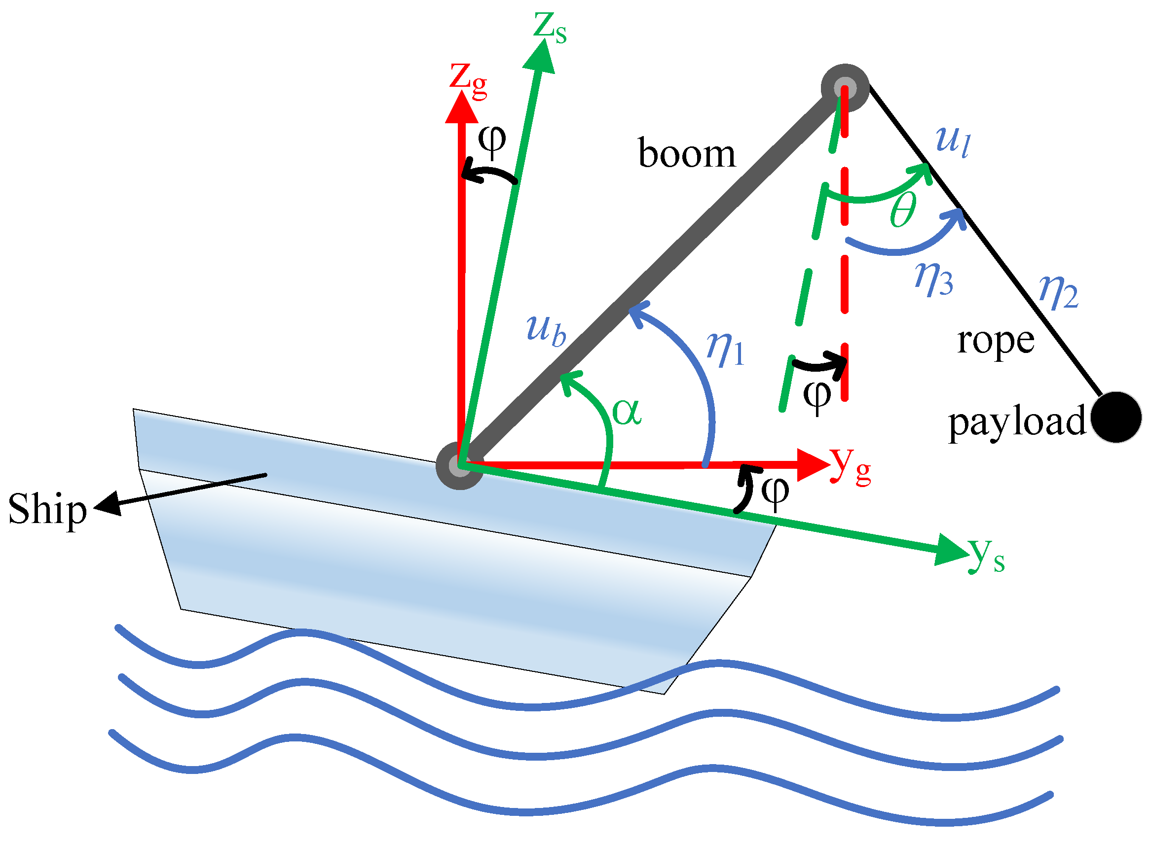
2.1. Dynamics for Shipboard Boom Cranes

The physical model of the shipboard boom crane system is shown in Figure 1, which introduces two coordination systems: the ground-fixed coordination system $y_g-O{-\mathrm{z}}_g$ and the ship-fixed coordination system $y_s-O{-\mathrm{z}}_s$. The variables and parameters of the system are shown in Table 1. The corresponding dynamic equation can be expressed in the following Lagrange’s form [30]:

$$M(q)\ddot{q}+C(q,\dot{q})\dot{q}+G(q)=u+{\tau }_d$$

(1)

where $q={[\begin{array}{ccc}\alpha & l& \theta \end{array}]}^{\top }\in {ℝ}^{3\times 1}$ is the state vector, $M(q)\in {ℝ}^{3\times 3}$ and $V(q,\dot{q})\in {ℝ}^{3\times 3}$ denote the inertia and centripetal-Coriolis matrices, respectively, $G(q)\in {ℝ}^{3\times 1}$ represents the gravity vector, $u={[\begin{array}{ccc}{u}_b& u_l& 0\end{array}]}^{\top }\in {ℝ}^{3\times 1}$ and ${\tau }_d\in {ℝ}^{3\times 1}$ represent the control input vector and perturbation vector, respectively. All elements contained in aforesaid matrices and vectors are given as

$$M=\left[\begin{array}{ccc}J+m_c{b}^2& -m_{c}b{C}_{\theta -\alpha }& m_{c}bl{S}_{\theta -\alpha }\\ -m_{c}b{C}_{\theta -\alpha }& m_c& 0\\ m_{c}bl{S}_{\theta -\alpha }& 0& m_c{l}^2\end{array}\right],$$

(2)

$$C=\left[\begin{array}{ccc}0& m_{c}b{S}_{\theta -\alpha }\dot{\theta }& c_{13}\\ -m_{c}b{S}_{\theta -\alpha }\dot{\alpha }& 0& -m_{c}l\dot{\theta }\\ -m_{c}bl{C}_{\theta -\alpha }\dot{\alpha }& m_{c}l\dot{\theta }& m_{c}l\dot{l}\end{array}\right],$$

(3)

$$G={[(m_{c}b+m_d)g{C}_{\alpha -\phi },-m_{c}g{C}_{\theta -\phi },m_{c}gl{S}_{\theta -\phi }]}^{\top },$$

(4)

$$\tau ={\left[\begin{array}{c}(J+m_c{b}^2+m_{c}bl{S}_{\theta -\alpha })\ddot{\phi }+2m_{c}b\dot{l}{S}_{\theta -\alpha }\dot{\phi }-m_{c}bl{C}_{\theta -\alpha }({\dot{\phi }}^2-2\dot{\theta }\dot{\phi })\\ m_{c}l({\dot{\phi }}^2-2\dot{\theta }\dot{\phi })+m_{c}b{S}_{\theta -\alpha }({\dot{\phi }}^2-2\dot{\alpha }\dot{\phi })-m_{c}b{C}_{\theta -\alpha }\ddot{\phi }\\ m_{c}l(b{S}_{\theta -\alpha }+l)\ddot{\phi }+m_{c}bl{C}_{\theta -\alpha }({\dot{\phi }}^2-2\dot{\alpha }\dot{\phi })+2m_{c}l\dot{l}\dot{\phi }-{\tau }_r(\dot{\theta }-\dot{\phi })\end{array}\right]}^{\top },$$

(5)

where $c_{13}=mb(S_{\theta -\phi }\dot{l}+l{C}_{\theta -\phi }\dot{\theta })$,${\tau }_r\in {ℝ}^{+}$ represents the damping coefficient. In addition, the symbols $S_{a-b}$ and $C_{a-b}$ ($a,b=\alpha ,\beta ,\phi$) represent functions $\sin (a-b)$ and $\cos (a-b)$, respectively.

As shown in Figure 1, the desired position of the payload in the ground-fixed coordination system is:

$$\begin{array}{l}{y}_d=b\cos ({\alpha }_d-\phi )+l_d\sin ({\theta }_d-\phi ),\\ z_d=b\sin ({\alpha }_d-\phi )-l_d\cos ({\theta }_d-\phi ),\end{array}$$

(6)

where ${\alpha }_d$, ${\theta }_d$, and $l_d$ represent the desired boom luffing angle, rope length, and payload swing angle, respectively. To fully accomplish the task of suppressing payload swing, it is straightforward to deduce that ${\theta }_d=\phi (t)$. Therefore, we can derive the following:

$$\begin{array}{l}{a}_d=\phi +arc\cos ({\displaystyle \frac{y_d}{b}}),\\ l_d=\sqrt{b^2-y_d^2}-z_d,{\theta }_d=\phi .\end{array}$$

(7)

It can be observed that ${\alpha }_d$, ${\theta }_d$, and $l_d$ are time-varying, which poses significant challenges in controller design. To facilitate subsequent analysis and simplify calculations, we construct the following new state variables:

$$\eta ={[\begin{array}{ccc}{\eta }_1& {\eta }_2& {\eta }_3\end{array}]}^{\top }={[\begin{array}{ccc}\alpha -\phi & l& \theta -\phi \end{array}]}^{\top }.$$

(8)

Together with equations (7) and (8), the desired values of the new state variables ${\eta }_1$, ${\eta }_2$, and ${\eta }_3$ can be expressed as:

$${\eta }_{1d}=\arccos ({\displaystyle \frac{y_d}{b}}),{\eta }_{2d}=\sqrt{b^2-y_d^2}-z_d,{\eta }_{3d}=0.$$

(9)

As shown in (9), the newly constructed state variables eliminate the ship's roll angle from (6), making the subsequent controller design more convenient and straightforward. Correspondingly, equations (1)-(5) can be transformed into:

$$M(\eta )\ddot{\eta }+C(\eta ,\dot{\eta })\dot{\eta }+G(\eta )=u+{\tau }_{dn}$$

(10)

$$M=\left[\begin{array}{ccc}J+m_c{b}^2& -m_{c}b{C}_{1-3}& -m_{c}b{\eta }_2{S}_{1-3}\\ -m_{c}b{C}_{1-3}& m_c& 0\\ -m_{c}b{\eta }_2{S}_{1-3}& 0& m_c{l}^2\end{array}\right],$$

(11)

$$C=\left[\begin{array}{ccc}0& -m_{c}b{S}_{1-3}{\dot{\eta }}_3& c_{n13}\\ m_{c}b{S}_{1-3}{\dot{\eta }}_1& 0& -m_c{\eta }_2{\dot{\eta }}_3\\ -m_{c}b{\eta }_2{C}_{1-3}{\dot{\eta }}_1& m_c{\eta }_2{\dot{\eta }}_3& m_c{\eta }_2{\dot{\eta }}_2\end{array}\right],$$

(12)

$$G={[(m_{c}b+m_d)g{C}_1,-m_{c}g{C}_3,m_{c}gl{S}_3]}^{\top },$$

(13)

$${\tau }_{dn}={\left[\begin{array}{ccc}0& 0& -{\tau }_r{\dot{\eta }}_3\end{array}\right]}^{\top },$$

(14)

where $c_{n13}=mb(-S_{1-3}{\dot{\eta }}_2+{\eta }_2{C}_{1-3}{\dot{\eta }}_3)$, and the symbols $S_{i-j}$ and $C_{i-j}$ ($i,j=1,2,3$) represent the abbreviations of $\sin ({\eta }_i-{\eta }_j)$ and $\cos ({\eta }_i-{\eta }_j)$, respectively.

It can be verified that $M(\eta )$ in (11) has the following property [27]:

$$\begin{array}{cc}{x}^{\top }\left[{\displaystyle \frac{1}{2}}\dot{M}(\eta )-C(\eta ,\dot{\eta })\right]x=0,& \forall x\in {ℝ}^3\end{array}.$$

(15)

In practice, the initial values of the new state variables are within the preset ranges, i.e.,

$$\begin{array}{l}-{\displaystyle \frac{\pi }{2}}<m_1<{\eta }_1(0)<M_1<{\displaystyle \frac{\pi }{2}}, \\ 0<m_2<{\eta }_2(0)<M_2,\\ -{\displaystyle \frac{\pi }{2}}<m_3<{\eta }_3(0)<M_3<{\displaystyle \frac{\pi }{2}},\end{array}$$

(16)

where, $m_i,i=1,2,3$ and $M_i,i=1,2,3$ represent the state variables' allowable minimum and maximum values, respectively. For instance, $m_2$ and $M_2$ denote the permissible shortest and longest cable lengths greater than zero to comply with practical operational requirements.

2.2. Control Objective

For the system (10), we aim to design an appropriate controller $u$ to achieve the following objectives:

In the fixed ground coordinate system, transport the payload from its initial position to its desired position while eliminating residual payload swing, that is, make the new output state vector $\eta$ converge to its desired value ${\eta }_d$, which is expressed as:

$$\underset{t\to \infty }{\lim }{\eta }_1={\eta }_{1d}, \underset{t\to \infty }{\lim }{\eta }_2={\eta }_{2d}, \underset{t\to \infty }{\lim }{\eta }_3={\eta }_{3d}.$$

(17)

Considering the operational safety, limited workspace, and other specific requirements, the system's new output state vector $\eta$ is constrained within the preset range throughout the operation, which can be described as:

$$\left\{\begin{array}{cc}\begin{array}{l}-{\displaystyle \frac{\pi }{2}}<m_1<{\eta }_1(t)<M_1<{\displaystyle \frac{\pi }{2}},\\ 0<m_2<{\eta }_2(t)<M_2,\\ -{\displaystyle \frac{\pi }{2}}<m_3<{\eta }_3(t)<M_3<{\displaystyle \frac{\pi }{2}},\end{array}& \forall \mathrm{t}\ge 0\end{array}\right..$$

(18)

3. Controller Design and Stability Analysis

In this section, a novel and effective controller is designed to achieve the objective above, and its effectiveness is rigorously demonstrated through theoretical analysis.

3.1. Controller Design

First, based on (9) and (17), the following error signals are defined:

$$e_1={\eta }_1-{\eta }_{1d}, e_2={\eta }_2-{\eta }_{2d}, e_3={\eta }_3-{\eta }_{3d}={\eta }_3,$$

(19)

correspondingly

$${\dot{e}}_1={\dot{\eta }}_1, {\dot{e}}_2={\dot{\eta }}_2, {\dot{e}}_3={\dot{\eta }}_3.$$

(20)

Second, the storage energy of the shipboard crane system reads as

$$E_0={\displaystyle \frac{1}{2}}{\dot{\eta }}^{\top }{\rm M}(\eta )\dot{\eta }+m_{c}g{\eta }_2[1-\cos ({\eta }_3)]$$

(21)

Based on this, we replace $q$, $l$, and $\theta$ in (20) with $\eta$, ${\eta }_2$, and ${\eta }_3$, respectively, to obtain the following storage function:

$$E_0={\displaystyle \frac{1}{2}}{\dot{\eta }}^{\top }{\rm M}(\eta )\dot{\eta }+m_{c}g{\eta }_2[1-\cos ({\eta }_3)]$$

(22)

Then, differentiating $E_0$ and substituting Error! Reference source not found. into the result produces

$$\begin{array}{c}{\dot{E}}_0=[u_b-(m_{c}b+m_d)g{C}_1]{\dot{\eta }}_1+\\ (u_l+m_{c}g){\dot{\eta }}_1-{\tau }_r{\dot{\eta }}_3^2\end{array}$$

(23)

where property (15) has been used.

To fulfill the output state constraints, following auxiliary variables are constructed:

$$\begin{array}{c}{r}_b(e_1)=e_1\log [({\eta }_1-m_1)/(M_1-{\eta }_1)]\{(M_1-m_1)e_1/[({\eta }_1-m_1)(M_1-{\eta }_1)]\\ +\log [({\eta }_1-m_1)/(M_1-{\eta }_1)]\},\end{array}$$

(24)

$$\begin{array}{c}{r}_l(e_2)=e_2\log [({\eta }_2-m_2)/(M_2-{\eta }_2)]\{(M_2-m_2)e_2/[({\eta }_2-m_2)(M_2-{\eta }_2)]\\ +\log [({\eta }_2-m_2)/(M_2-{\eta }_2)]\},\end{array}$$

(25)

$$r_u({\eta }_3)=\log [({\eta }_3-m_3)/(M_3-{\eta }_3)],$$

(26)

where $\log$ stands for natural logarithm function.

In general, appropriately enhancing the dynamic coupling between the boom and the payload facilitates damping injection, and one possible approach is to combine them into a composite signal [9]. To achieve this, based on (26), a new composite signal is constructed as follows:

$$r_{\psi }({\dot{\eta }}_1,{\eta }_3,{\dot{\eta }}_3)=k_{r3}[r_u+\sin ({\eta }_3)+\cos ({\eta }_3){\dot{\eta }}_3]+k_a{\dot{\eta }}_1$$

(27)

where $k_{r3}$ and $k_a$ are positive constants.

Therefore, in order to effectively constrain the system motion and utilize the designed coupling characteristics (27) to improve the system transient performance, we design the following controller:

$$\begin{array}{c}{u}_b=-k_{p1}{e}_1-k_{d1}{\dot{\eta }}_1+(m_{c}b+m_d)g{C}_1\\ -k_{r1}{r}_b-r_{\psi }\varpi ,\\ u_l=-k_{p2}{e}_2-k_{d2}{\dot{\eta }}_2-m_{c}g-k_{r2}{r}_l,\end{array}$$

(28)

with

$$\dot{\varpi }=-\varpi +r_{\psi }{\dot{\eta }}_1,$$

(29)

where $k_{p1},k_{d1},k_{p2},k_{d2},k_{r1},k_{r2}\in {ℝ}^{+}$ are positive control gains to be adjusted.

Note that the controller proposed in (28) does not exhibit singularity, which will be proven in the subsequent stability analysis section.

Remark 1.

This paper proposes a novel barrier function to address the issue of asymmetric output constraints in nonlinear systems, such as the constraint on the boom luffing angle in (24), the constraint on cable length in (25), and the constraint on the swing angle of the underactuated payload in (27). Notably, unlike conventional approaches to handling underactuated state constraints [28,32], this study embeds the relevant constraint term (27) into the controller by constructing an auxiliary signal (29), which significantly simplifies the complexity of controller design and provides valuable insights for designing controllers and applying them in practice in future work. Moreover, the constructed auxiliary signal intentionally strengthens the dynamic coupling between the boom and the payload, further enhancing the damping effect on the payload swing.

Remark 2.

Inspired by the tuning rules of PID controllers, the control gains k_p1, k_d1, k_p2, and k_d2 in the proposed controller can be appropriately selected. Additionally, k_r1, k_r2, k_r3, and k_a associated with the auxiliary constraint terms, can be set as small positive values through a straightforward trial-and-error approach.

3.2. Stability Analysis

Theorem 1.

Under the continuous ship motion caused by sea wave effects, the proposed controller (28) ensures that the system satisfies the constraints in (18) and achieves the control objective described in (17).

Proof of Theorem 1.

Based on (22), we choose

$$\begin{array}{cc}V=& E_0+{\displaystyle \frac{1}{2}}{k}_{p1}{e}_1^2++{\displaystyle \frac{1}{2}}{\varpi }^2+{\displaystyle \frac{1}{2}}{k}_{p2}{e}_2^2+{\displaystyle \frac{1}{2}}{k}_{r1}\{\log [({\eta }_1-m_1)/(M_1-{\eta }_1)]e_1\}2\\ & +{\displaystyle \frac{1}{2}}{k}_{r2}\{\log [({\eta }_2-m_2)/(M_2-{\eta }_2)]e_2\}2.\end{array}$$

(30)

Then, by taking the time derivative of (30) and considering (23), we obtain:

$$\dot{V}=[u_b+k_{p1}{e}_1-(m_{c}b+m_d)g{C}_1+k_{r1}{r}_b]{\dot{\eta }}_1+[u_l+m_{c}g+k_{p2}{e}_2+k_{r2}{r}_l]{\dot{\eta }}_2-{\tau }_r{\dot{\eta }}_3^2+\varpi \dot{\varpi }.$$

(31)

By substituting the results of (28) and (29) into (31), one can yield that

$$\dot{V}=-k_{d1}{\dot{\eta }}_1^2-{\varpi }^2-k_{d2}{\dot{\eta }}_2^2-{\tau }_r{\dot{\eta }}_3^2.$$

(32)

Obviously

$$\dot{V}\le 0,$$

(33)

which indicates that

$$V(t)\le V(0)\ll +\infty .$$

(34)

Furthermore, we can prove the following two items through (34):

4.

Assume that ${\eta }_1$ and ${\eta }_2$ reach their preset upper or lower limits at time $T$. In this case, the logarithmic terms corresponding to these variables in $V$ would tend to infinity, leading to $V(T)$ being infinite. This conclusion contradicts the fact stated in (34). By reduction to absurdity, the state variables ${\eta }_1$ and ${\eta }_2$ are always able to comply with their constraints, that is:

$$-{\displaystyle \frac{\pi }{2}}<m_1<{\eta }_1<M_1<{\displaystyle \frac{\pi }{2}}, 0<m_2<{\eta }_2<M_2$$

(35)

5.

Assuming that ${\eta }_3$ violates any constraint within a very small adjacent time $t\in [T_1,T_2]$, referring to (26) and (27), $r_{\psi }$ will be infinite. And for $t\in [T_1,T_2]$, the solution of the differential equation (29) is

$$\varpi (T_2)=\varpi (T_1)e^{-(T_2-T_1)}+{\displaystyle {\int }_{T_1}^{T_2}{r}_{\psi }(\rho ){\dot{\eta }}_1(\rho )e^{-(T_2-\rho )}d\rho }\to \infty ,as {\eta }_3\to m_3 or{ \mathrm{M}}_3,$$

(36)

this result contradicts the fact stated in (34). Once again, by reduction to absurdity, the state variable ${\eta }_3$ is always able to comply with its constraints, that is:

$$-{\displaystyle \frac{\pi }{2}}<m_3<{\eta }_3<M_3<{\displaystyle \frac{\pi }{2}}$$

(37)

Considering the results of (35) and (37), the new state vector $\eta$ always satisfies its preset constraints, i.e., the objective described in (18). These results also show that the proposed controller will not have singularities and

$$V\ge 0$$

(38)

From (34) to (38), it is not difficult to see that

$$\begin{array}{l}V(t)\in L_{\infty }\to {\dot{\eta }}_1,{\dot{\eta }}_2,{\dot{\eta }}_3,e_1,e_2,e_3,\log [({\eta }_1-m_1)/(M_1-{\eta }_1),\\ \log [({\eta }_2-m_2)/(M_2-{\eta }_2),\varpi \in L_{\infty }.\end{array}$$

(39)

Then, according to the controller formulas expressed in (24)-(28), we can infer

$$u_b,u_l\to L_{\infty }$$

(40)

Substituting the results of (39) and (40) into formula (10), we obtain

$${\ddot{\eta }}_1,{\ddot{\eta }}_2,{\ddot{\eta }}_3\in L_{\infty }$$

(41)

Next, we discuss the stability of system (10) with the controller (28) by using LaSalle invariance theorem [33]. let $\Phi$ be the largest invariant set in $\Xi$, where

$$\Xi =\{\eta ,\dot{\eta }|\dot{V}=0\}.$$

(42)

Then, from the results of (32) and (33), one can conclude that in $\Phi$

$${\dot{\eta }}_1,{\dot{\eta }}_2,{\dot{\eta }}_3,\varpi =0\to {\ddot{\eta }}_1,{\ddot{\eta }}_2,{\ddot{\eta }}_3=0.$$

(43)

Substituting (43) into (10) and using the results of (13), (14), and (28), we obtain

$$\begin{array}{c}-k_{p1}{e}_1-k_{r1}{r}_b(e_1)=0\to e_1=0,\\ -k_{p2}{e}_2-k_{r2}{r}_l(e_2)=m_{c}g(1-C_3),\\ m_{c}gl{S}_3=0.\end{array}$$

(44)

According to the result of (37) and the property of the sine function, we can infer that

$$S_3=0\to {\eta }_3=0,e_3=0.$$

(45)

Hence

$$-k_{p2}{e}_2-k_{r2}{r}_l(e_2)=m_{c}g(1-C_3)=0\to e_2=0.$$

(46)

From equations (43)-(46), we know that the largest invariant set $\Xi$ includes only the equilibrium point. Hence, states $\eta$ and $\dot{\eta }$ converge asymptotically to their desired values. Finally, by combining the results of (35) and (37), Theorem 1 is proved.□

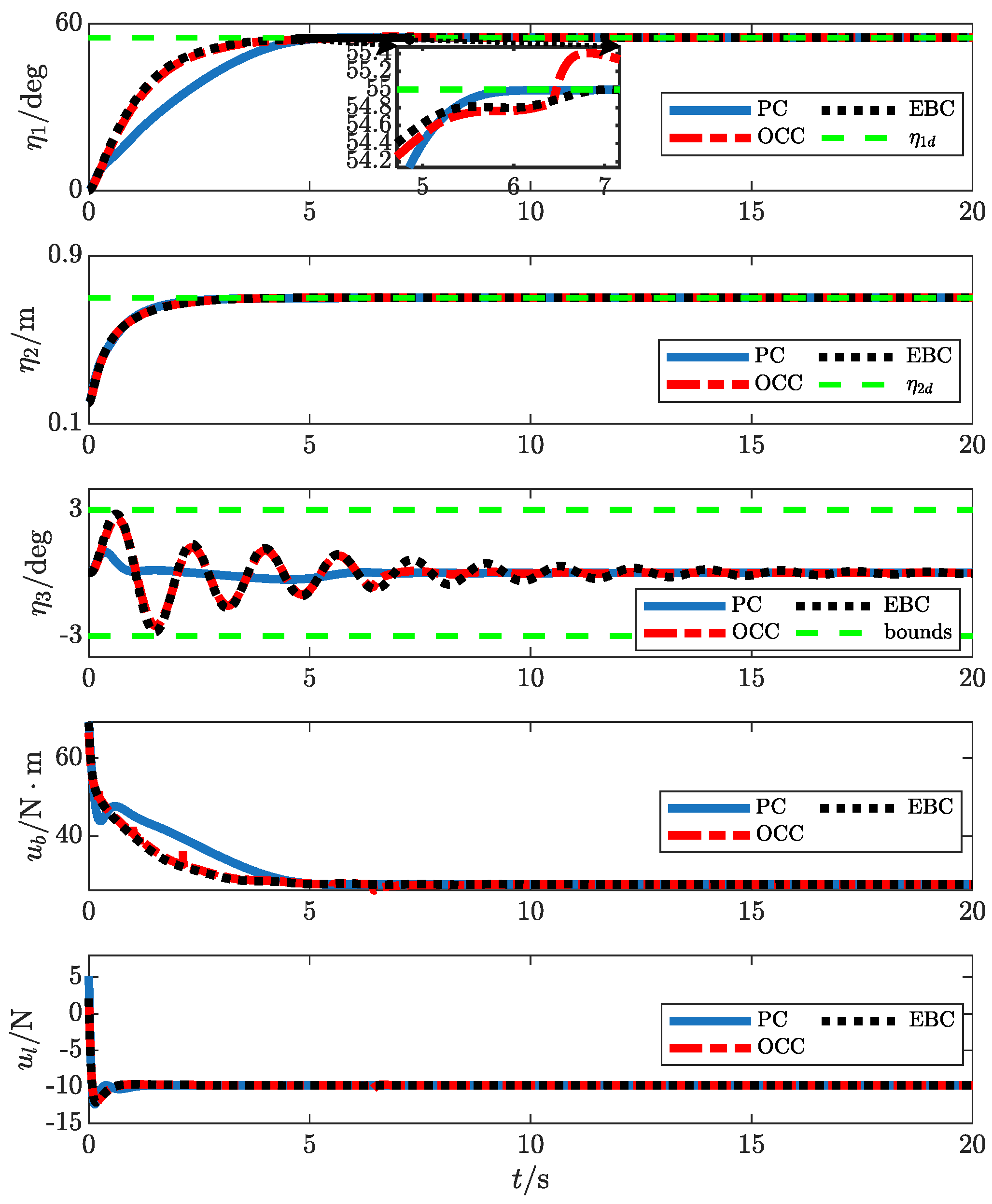
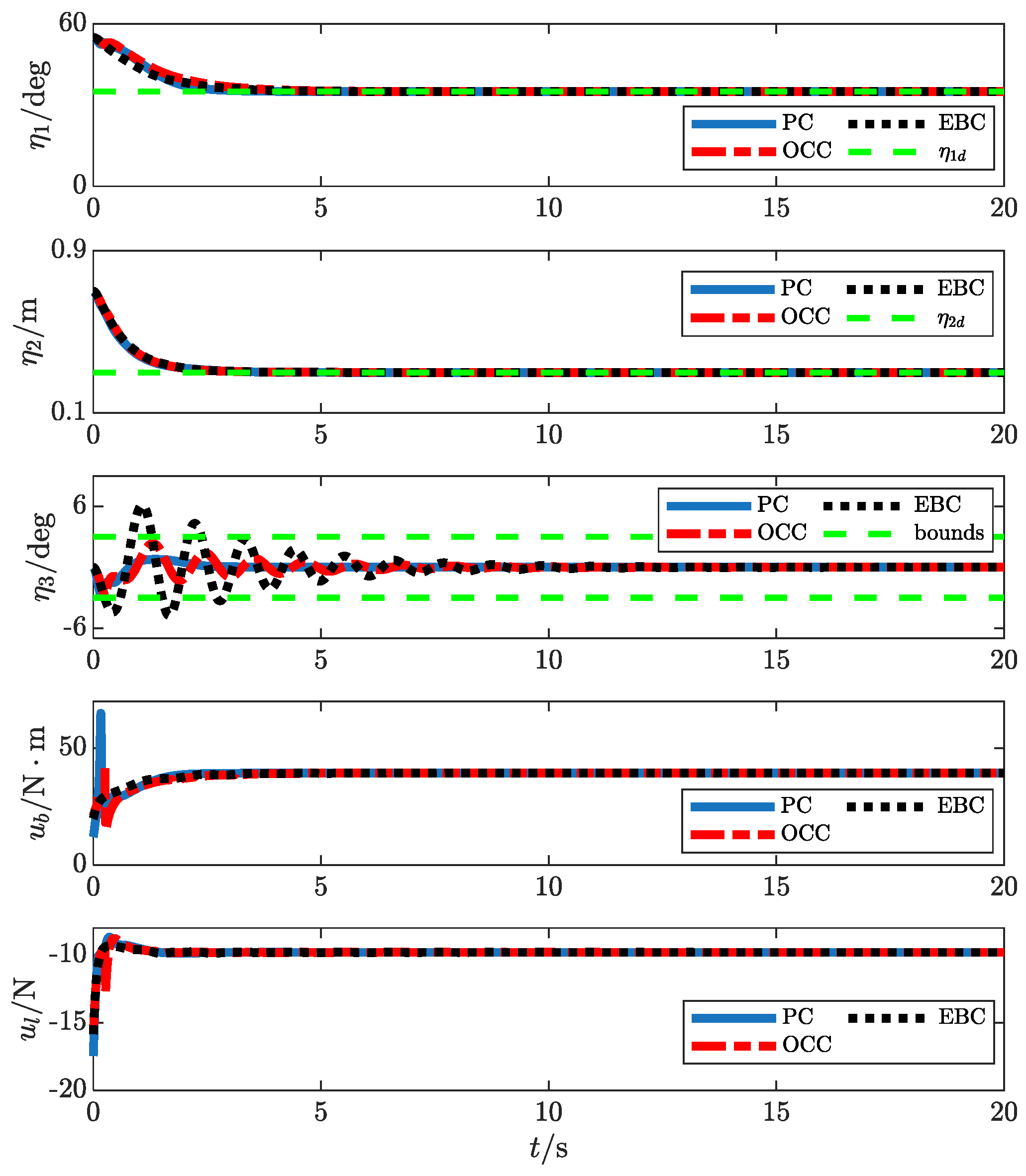
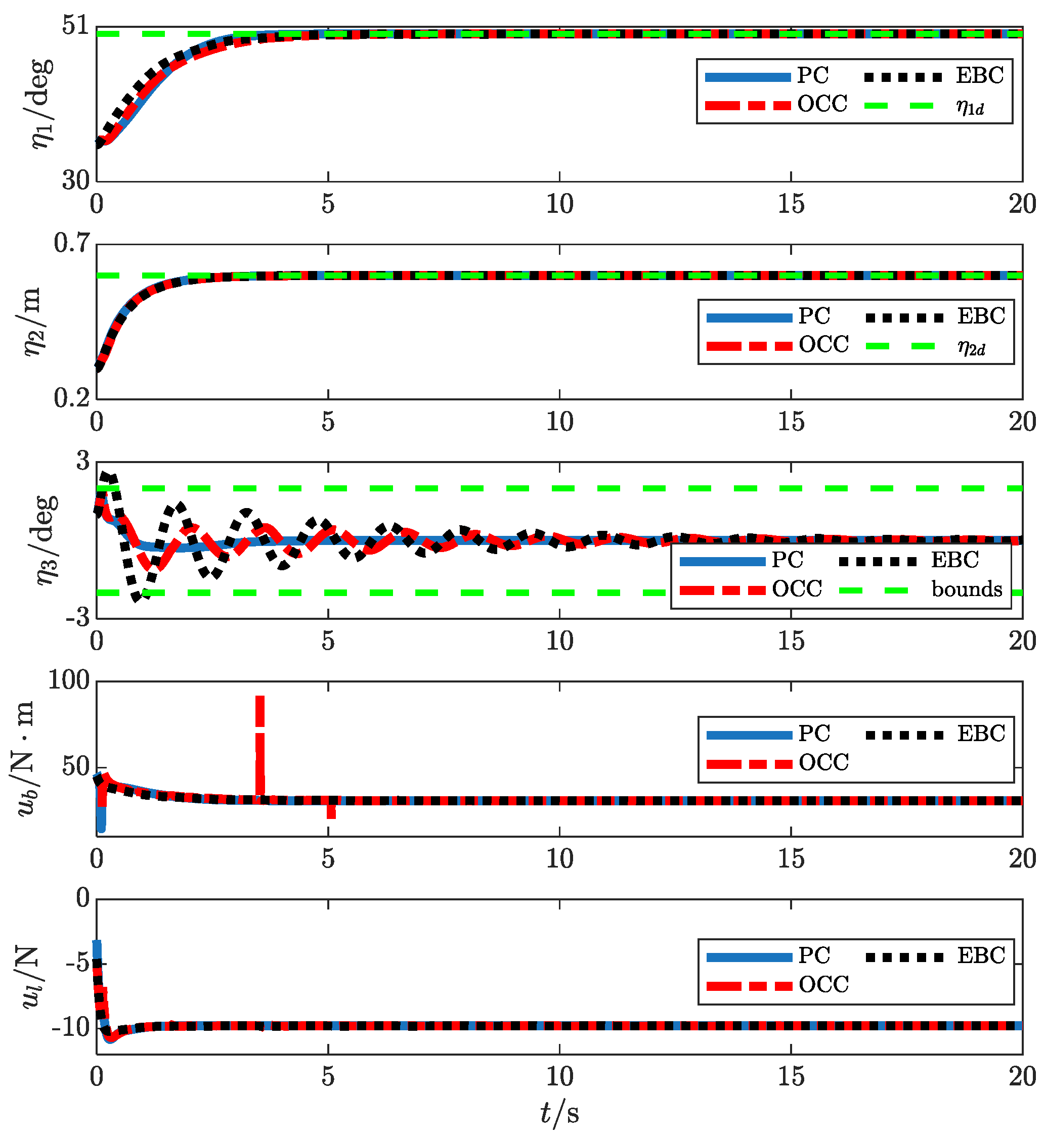
4. Simulation Results

To verify the effectiveness and evaluate the performance of the proposed controller in (28), we set up three simulations based on the MATLAB/SIMULINK platform, with a simulation sampling time $5 \mathrm{ms}$.

In simulations, to thoroughly verify the effectiveness and performance of the proposed controller, we selected the existing advanced nonlinear anti-swing control methods [30,32] for shipboard boom cranes as comparison objects. Among them, the energy-based controller [30] is similar to PD control and has typical control performance, so the comparison results can intuitively reflect the control effect of the proposed controller; the controller with output constraints [32] has the ability to process symmetrical constraints of output states, which is in sharp contrast to the asymmetric output constraints processing ability of the proposed method, thereby further verifying the advantage of the proposed controller in constraints processing and the transient performance improvement effect brought by this advantage. For the convenience of description, we will mark the energy-based controller [30] as EBC, the controller with output constraints [32] as OCC, and the proposed controller as PC.

Then, relying on the MATLAB/SIMULINK platform, three groups of simulations are designed to verify the effectiveness of the proposed control method. The corresponding simulation results are shown in Figure 2, Figure 3 and Figure 4 and some specific quantified results are listed in Table 2, Table 3 and Table 4 where the performance indices are defined as follows:

6.

$t_p$: The time taken for the rope length’s positioning error converging to the range of $(-0.004 \mathrm{m},0.004 \mathrm{m})$.

7.

${\eta }_{3\max }$: The maximum amplitude of payload swing during control.

8.

$t_c$: The time taken for the payload swing angle converging to the range of $(-0.04°,0.04°)$.

Group 1.

Performance Comparison. To intuitively reflect the performance of the proposed controller (28), we compare it with EBC and OCC without any disturbances. The simulation parameters are set as follows:

The main physical parameters of the shipboard crane system are:

$$\begin{array}{l}{m}_c=1.0 \mathrm{kg}, \mathrm{b}=0.9 \mathrm{m}, m_d=4.0 \mathrm{kg}\cdot \mathrm{m},\\ J=2.7 \mathrm{kg}\cdot {\mathrm{m}}^2,g=9.8, {\tau }_r=\mathrm{0.05.}\end{array}$$

The initial values and desired values of the system states are selected as:

$$\begin{array}{l}{\eta }_1(0)=0\mathrm{deg},{\eta }_2(0)=0.1 \mathrm{m}, {\eta }_3(0)=0,\\ {\eta }_{1d}=55\mathrm{deg}, {\eta }_{2d}=0.7 \mathrm{m}, {\eta }_{3d}=0 \mathrm{deg}.\end{array}$$

The state constraints are defined as:

$$\begin{array}{l}{\eta }_1\in (-55 \mathrm{deg}, 60\mathrm{deg}), {\eta }_2\in (0.1 \mathrm{m}, 0.9 \mathrm{m}),\\ {\eta }_3\in (-3 \mathrm{deg}, 3\mathrm{deg}).\end{array}$$

To achieve better control performance, after careful tuning, the control parameters for EBC are selected as:

$$k_{p1}=22, k_{d1}=25, k_{p2}=15, k_{d2}=11, \lambda =\mathrm{0.05.}$$

The control parameters of OCC are:

$$\begin{array}{l}{k}_{p\eta 1}=21, k_{d\eta 1}=25, k_{\delta }=0.005, k_3=0.00001, \\ k_{p\eta 2}=15, k_{d\eta 2}=11, k_l=0.05, {\delta }_{\eta 1}=5, {\eta }_{3r}=3.\end{array}$$

The control parameters of PC are:

$$\begin{array}{l}{k}_{p1}=22, k_{d1}=21, k_{r1}=1, k_{r3}=6, k_a=16, k_{p2}=15,\\ k_{d2}=11, k_{r2}=1, M_1=60 \mathrm{deg}, m_1=-55 \mathrm{deg}, \\ M_2=0.9{ \mathrm{m}, \mathrm{m}}_2=0.1 \mathrm{m}, M_3=3\mathrm{deg}, m_3=-3 \mathrm{deg},\end{array}$$

The simulation results for Group 1 are shown in Figure 2, with the corresponding quantified results provided in Table 2. It can be seen that all controllers make the new states converge to their desired values asymptotically without violating the preset constraints in the process, and the boom luffing angle and rope length do not overshoot. Based on the performance indicators, the proposed controller has better control performance than EBC and OCC. Specifically, when the boom luffing angle and rope length converge at almost the same time in all controllers, the maximum payload swing angle under the proposed controller is the smallest, which is $1°$; in addition, the payload swing angle is also quickly suppressed, converging to its expected range in the shortest time of $5.7 \mathrm{s}$, and there is no residual swing. In contrast, the maximum load swing angle under OCC control and EBC control is larger for both, and the time they take to converge the payload swing angle to its desired range is longer for both. Particularly, the time EBC takes is more than $20 \mathrm{s}$, mainly because it relies on natural damping to eliminate residual swing because the controller does not contain load swing angle information. This fact also reflects the advantages of the auxiliary signal constructed in this paper. This fact also reflects the advantages of the auxiliary signal constructed in this paper. It not only introduces the swing angle-related constraint term to ensure the asymmetric constraint and thus improve the transient performance but also cleverly couples the boom amplitude change speed and many swing angle-related information to further improve the coordinated control capability.

Group 2.

Robustness comparison. In order to verify the robustness of the proposed controller under different transportation conditions, this simulation will change the states' initial and expected values. Specifically, we use the expected values of the states set in the last simulation as the initial values of the states in this simulation, that is, ${\eta }_1(0)=55\mathrm{deg}, {\eta }_2(0)=0.7 \mathrm{m}, {\eta }_3(3)=0 \mathrm{deg}$, and then set the expected values of the states to${\eta }_{1d}=35\mathrm{deg}, {\eta }_{2d}=0.3 \mathrm{m}, {\eta }_{3d}=0 \mathrm{deg}$, and other control parameters and system parameters remain unchanged.

The simulation results of Group 2 are shown in Figure 3, with the quantized data provided in Table 3. Similarly, all the new states quickly and asymptotically converge to their desired values. For controlling the boom luffing angle and rope length, the three controllers exhibit similar control performance, with no overshoot and roughly equivalent convergence times. In terms of other performance indicators, the proposed controller shows satisfactory positioning and anti-swing performance. The payload swing angle converges to its desired range in the fastest time of $3.2 \mathrm{s}$, with no residual swing, and the maximum swing amplitude is limited to $2.7°$. In contrast, the control performance of OCC and EBC declines progressively. Specifically, regarding the control of the payload swing angle, OCC adheres to the predetermined constraints, but the convergence time is slower than the proposed controller's. EBC, on the other hand, not only severely violates the predetermined constraints, with the maximum swing amplitude reaching twice the upper limit, but also takes the longest time for the payload swing angle to converge to its expected range.

Group 3.

Stricter Constraints. In practical applications, due to factors such as inertia and friction, the payload swing angle often has an initial non-zero value, which presents a challenge for improving control performance. In this scenario, the preset constraints must still be satisfied to ensure operational safety and enhance transport efficiency. Therefore, we further tightened all output constraints under non-zero initial conditions to verify the proposed controller's strong performance in handling output constraints.

Therefore, we set the system's initial conditions as ${\eta }_1(0)=35\mathrm{deg}, {\eta }_2(0)=0.3 \mathrm{m}, {\eta }_3(3)=1 \mathrm{deg}$, with the states' desired values as ${\eta }_{1d}=50\mathrm{deg}, {\eta }_{2d}=0.6 \mathrm{m}, {\eta }_{3d}=0 \mathrm{deg}$. The stricter constraint settings are ${\eta }_1\in (30 \mathrm{deg}, 51\mathrm{deg}),{\eta }_2\in (0.2 \mathrm{m}, 0.7 \mathrm{m}),{\eta }_3\in (-2 \mathrm{deg}, 2\mathrm{deg})$. Apart from adjusting the parameters related to constraints, such as $M_i,m_i,i=1,2,3$ in the PC controller and ${\delta }_{\eta 1}, {\eta }_{3r}$ in the OCC controller according to the constraints, other control parameters and system parameters remain unchanged.

Group 3's simulation results and their quantified data are shown in Figure 4 and Table 4, respectively. In terms of cable length control, the performance of all three controllers is nearly identical. However, in the control of the other two states, the proposed controller demonstrates clear advantages. Specifically, both the boom luffing angle and payload swing angle converge to their desired values in the shortest time, and under non-zero initial conditions, the maximum payload swing angle not only satisfies the contracted constraints but also achieves the smallest swing( $1.8°$) among the three controllers. In contrast, both OCC and EBC have significant disadvantages: OCC shows sharp spikes in boom luffing angle control, which could impact the motor's lifespan, and EBC fails to keep the payload swing angle within the preset constraints while also taking much longer to converge to the desired swing angle range compared to the proposed controller. Therefore, even with non-zero initial values and changes in desired values and constraints, the proposed controller still provides superior transient performance and robustness.

5. Conclusions

This paper develops a nonlinear anti-sway control method for underactuated ship-mounted cranes featuring excellent capability in handling asymmetric output constraints. Specifically, after model transformation, an energy-based controller ensuring asymptotic stability is first established using BLFs. Notably, the proposed BLF successfully addresses constraints with same signs for the rope length by modifying the traditional symmetric BLF. To handle the constraints of underactuated states, an auxiliary signal is introduced, allowing the modified BLF to be cleverly embedded into the controller. To enhance the system's anti-sway performance further, the auxiliary signal fully couples the boom luffing velocity and payload swing angle information, enabling more refined coordination control. Finally, based on the system's energy function, the stability of the closed-loop system is theoretically proven using the Lyapunov method, and the effectiveness of the proposed controller is validated through numerical simulations. In the future, we will comprehensively consider system parameter uncertainties and output constraints to promote the practical application of the proposed method in ship-mounted cranes.

References

1. Küchler, S.; Mahl, T.; Neupert, J.; Schneider, K.; Sawodny, O. Active control for an offshore crane using prediction of the vessel’s motion. IEEE/ASME transactions on mechatronics 2010, 16, 297–309. [Google Scholar] [CrossRef]
2. Rong, B.; Rui, X.; Lu, K.; Tao, L.; Wang, G.; Yang, F. Dynamics analysis and wave compensation control design of ship’s seaborne supply by discrete time transfer matrix method of multibody system. Mechanical Systems and Signal Processing 2019, 128, 50–68. [Google Scholar] [CrossRef]
3. Shi, J.; Hu, M.; Zhang, Y.; Chen, X.; Yang, S.; Hallak, T.S.; Chen, M. Dynamic Analysis of Crane Vessel and Floating Wind Turbine during Temporary Berthing for Offshore On-Site Maintenance Operations. Journal of Marine Science and Engineering 2024, 12, 1393. [Google Scholar] [CrossRef]
4. Huang, J.; Wang, W.; Zhou, J. Adaptive control design for underactuated cranes with guaranteed transient performance: theoretical design and experimental verification. IEEE Transactions on Industrial Electronics 2021, 69, 2822–2832. [Google Scholar] [CrossRef]
5. Liu, Z.; Fu, Y.; Sun, N.; Yang, T.; Fang, Y. Collaborative antiswing hoisting control for dual rotary cranes with motion constraints. IEEE Transactions on Industrial Informatics 2021, 18, 6120–6130. [Google Scholar] [CrossRef]
6. Ramli, L.; Mohamed, Z.; Abdullahi, A.M.; Jaafar, H.I.; Lazim, I.M. Control strategies for crane systems: A comprehensive review. Mechanical Systems and Signal Processing 2017, 95, 1–23. [Google Scholar] [CrossRef]
7. Wang, T.; Lin, C.; Li, R.; Qiu, J.; He, Y.; Zhou, Z.; Qiu, G. Nonlinear enhanced coupled feedback control for bridge crane with uncertain disturbances: theoretical and experimental investigations. Nonlinear Dynamics 2023, 111, 19021–19032. [Google Scholar] [CrossRef]
8. Sun, N.; Fang, Y. New energy analytical results for the regulation of underactuated overhead cranes: An end-effector motion-based approach. IEEE Transactions on Industrial Electronics 2012, 59, 4723–4734. [Google Scholar] [CrossRef]
9. Sun, N.; Fang, Y.; Wu, X. An enhanced coupling nonlinear control method for bridge cranes. IET Control Theory & Applications 2014, 8, 1215–1223. [Google Scholar]
10. Zhang, S.; He, X.; Zhu, H.; Li, X.; Liu, X. PID-like coupling control of underactuated overhead cranes with input constraints. Mechanical Systems and Signal Processing 2022, 178, 109274. [Google Scholar] [CrossRef]
11. Wang, T.; Tan, N.; Qiu, J.; Zheng, Z.; Lin, C.; Wang, H. A novel model-free adaptive terminal sliding mode controller for bridge cranes. Measurement and Control 2023, 56, 1217–1230. [Google Scholar] [CrossRef]
12. Maghsoudi, M.; Ramli, L.; Sudin, S.; Mohamed, Z.; Husain, A.; Wahid, H. Improved unity magnitude input shaping scheme for sway control of an underactuated 3D overhead crane with hoisting. Mechanical systems and signal processing 2019, 123, 466–482. [Google Scholar] [CrossRef]
13. Chen, Q.; Cheng, W.; Liu, J.; Du, R. Partial state feedback sliding mode control for double-pendulum overhead cranes with unknown disturbances. Proceedings of the Institution of Mechanical Engineers, Part C: Journal of Mechanical Engineering Science 2022, 236, 3902–3911. [Google Scholar] [CrossRef]
14. Chen, H.; Fang, Y.; Sun, N. A swing constraint guaranteed MPC algorithm for underactuated overhead cranes. IEEE/ASME Transactions on Mechatronics 2016, 21, 2543–2555. [Google Scholar] [CrossRef]
15. Cao, Y.; Li, T. Review of antiswing control of shipboard cranes. IEEE/CAA Journal of automatica Sinica 2020, 7, 346–354. [Google Scholar] [CrossRef]
16. Ngo, Q.H.; Hong, K.-S. Sliding-mode antisway control of an offshore container crane. IEEE/ASME transactions on mechatronics 2010, 17, 201–209. [Google Scholar] [CrossRef]
17. Saghafi Zanjani, M.; Mobayen, S. Anti-sway control of offshore crane on surface vessel using global sliding mode control. International Journal of Control 2022, 95, 2267–2278. [Google Scholar] [CrossRef]
18. Kim, G.-H.; Hong, K.-S. Adaptive sliding-mode control of an offshore container crane with unknown disturbances. IEEE/ASME Transactions On Mechatronics 2019, 24, 2850–2861. [Google Scholar] [CrossRef]
19. Lu, B.; Fang, Y.; Lin, J.; Hao, Y.; Cao, H. Nonlinear antiswing control for offshore boom cranes subject to ship roll and heave disturbances. Automation in Construction 2021, 131, 103843. [Google Scholar] [CrossRef]
20. Sun, N.; Yang, T.; Chen, H.; Fang, Y. Dynamic feedback antiswing control of shipboard cranes without velocity measurement: theory and hardware experiments. IEEE Transactions on Industrial Informatics 2018, 15, 2879–2891. [Google Scholar] [CrossRef]
21. Wu, Y.; Sun, N.; Chen, H.; Fang, Y. New adaptive dynamic output feedback control of double-pendulum ship-mounted cranes with accurate gravitational compensation and constrained inputs. IEEE Transactions on Industrial Electronics 2021, 69, 9196–9205. [Google Scholar] [CrossRef]
22. Guo, B.; Chen, Y. Fuzzy robust fault-tolerant control for offshore ship-mounted crane system. Information Sciences 2020, 526, 119–132. [Google Scholar] [CrossRef]
23. Jang, J.H.; Kwon, S.-H.; Jeung, E.T. Pendulation reduction on ship-mounted container crane via TS fuzzy model. Journal of Central South University 2012, 19, 163–167. [Google Scholar] [CrossRef]
24. Yang, T.; Sun, N.; Chen, H.; Fang, Y. Neural network-based adaptive antiswing control of an underactuated ship-mounted crane with roll motions and input dead zones. IEEE Transactions on Neural Networks and Learning Systems 2019, 31, 901–914. [Google Scholar] [CrossRef] [PubMed]
25. Li, Z.; Chuanjing, H.; Liu, C. Radical Basis Neural Network Based Anti-swing Control for 5-DOF Ship-Mounted Crane. In Proceedings of the International Conference on Neural Computing for Advanced Applications; 2024; pp. 18–29. [Google Scholar]
26. Cao, Y.; Li, T.; Hao, L.-Y. Lyapunov-based model predictive control for shipboard boom cranes under input saturation. IEEE Transactions on Automation Science and Engineering 2022, 20, 2011–2021. [Google Scholar] [CrossRef]
27. Sun, M.; Ji, C.; Luan, T.; Wang, N. LQR pendulation reduction control of ship-mounted crane based on improved grey wolf optimization algorithm. International Journal of Precision Engineering and Manufacturing 2023, 24, 395–407. [Google Scholar] [CrossRef]
28. Chen, H.; Sun, N. Nonlinear control of underactuated systems subject to both actuated and unactuated state constraints with experimental verification. IEEE Transactions on Industrial Electronics 2019, 67, 7702–7714. [Google Scholar] [CrossRef]
29. Li, E.; Liang, Z.-Z.; Hou, Z.-G.; Tan, M. Energy-based balance control approach to the ball and beam system. International Journal of Control 2009, 82, 981–992. [Google Scholar] [CrossRef]
30. Lu, B.; Fang, Y.; Sun, N.; Wang, X. Antiswing control of offshore boom cranes with ship roll disturbances. IEEE Transactions on Control Systems Technology 2017, 26, 740–747. [Google Scholar] [CrossRef]
31. Qian, Y.; Hu, D.; Chen, Y.; Fang, Y.; Hu, Y. Adaptive neural network-based tracking control of underactuated offshore ship-to-ship crane systems subject to unknown wave motions disturbances. IEEE Transactions on systems, man, and cybernetics: systems 2021, 52, 3626–3637. [Google Scholar] [CrossRef]
32. Wang, Y.; Yang, T.; Zhai, M.; Fang, Y.; Sun, N. Ship-Mounted Cranes Hoisting Underwater Payloads: Transportation Control With Guaranteed Constraints on Overshoots and Swing. IEEE Transactions on Industrial Informatics 2023, 19, 9968–9978. [Google Scholar] [CrossRef]
33. Khalil, H.K. Nonlinear Systems Third Edition. Upper Saddle River Nj Prentice Hall Inc 2002. [Google Scholar]
Figure 1. Schematic model of the shipboard boom crane.
Preprints 142726 g001
Figure 2. Group 1 simulation results.
Preprints 142726 g002
Figure 3. Group 2 simulation results.
Preprints 142726 g003
Figure 4. Group 3 simulation results.
Preprints 142726 g004