
Submitted:
21 February 2024
Posted:
21 February 2024
You are already at the latest version
Abstract
Measurements of temperature and salinity in the Amazon River plume in the open ocean of the western tropical North Atlantic are considered. The measurements were carried out using the AML CTD probe in the upper layer and a flow-through system that measures salinity and turbidity of seawater while the vessel is on the way. Additionally, archive oceanographic data from the WOD18 database, data of satellite altimetry measurements (AVISO), and satellite salinity data from Aquarius and SMOS were used. It is shown that the width of the Amazon plume is about 300–400 km, the depth of desalination is from 50 to 100 m. Surface salinity decreases compared to the background (36 PSU) by 0.5 PSU in February and more than by 3 PSU in September during the period of maximum development of the plume, which is determined from satellite measurements of surface salinity. Lagrangian modeling of the back-in-time advection of passive markers simulating freshwater particles was carried out. It was shown that the source of fresh water in the measurement area is the discharge of the Amazon.
Keywords:
desalination of the surface layer
; intra-annual plume variability
; CTD casts
; continuous recording
; Lagrangian analysis
1. Introduction
The Amazon is the largest river on our planet. The discharge of the Amazon River is estimated at 0.2 Sv (annual mean discharge is about 209,000 m3/s) [1,2,3]. A plume of desalinated Amazon water spreads across the entire tropical Atlantic. According to the results of recent studies [4], the dynamics of the Amazon plume significantly affects the regime of the entire equatorial Atlantic Ocean [5,6] (at least within the square 60° – 24°W and 5°S – 16°N), reducing surface salinity by 3–8 PSU (depending on the travelled distance from the delta) and the thickness of the upper quasi-homogeneous layer by 20–50 m, and also reducing the heat content of the ocean due to the “barrier effect” even at a great distance from the river mouth (up to 4,000 km and beyond).
The existence of the plume enhances the eastern transport of currents. The quantitative aspects of this influence remain poorly understood. The influence of Amazon waters is felt far from the river mouth as an increase in surface stratification due to desalination of the upper layer [7]. The Amazon River plume appears to contribute to atmosphere-ocean climate interaction dynamics in the western tropical North Atlantic. The flow of fresh water from the Amazon into the ocean does not only lead to climate changes in the region. The river carries coastal sediments, nutrients, and colored and transparent dissolved organic matter (CDOM, DOM) into the ocean, which are recorded as far as the coast of Africa [7]. Their entry leads to the development of phytoplankton cells and to an increase in the concentration of chlorophyll-a [8]. It was shown in [9] that the interaction of biota with nutrients in the plume leads to the absorption of atmospheric carbon dioxide by the waters of the river plume.
It was reported in [10] that variations in the Amazon River discharge influence the hydrological cycle, which is increasing river flows during the wet season and reduced water levels during the dry season observed since 2009. This phenomenon can affect the surface salinity of the tropical Atlantic. The authors propose a model to explain how the ocean, atmosphere, and the Amazon forest interact to cause this hydrological intensification.
Korosov with coauthors [11] analyzed spreading of the Amazon plume suggesting a synergistic tool based on an algorithm for deriving sea surface salinity from MODIS reflectance data together with sea surface salinity data from the SMOS and Aquarius satellites and the TOPAZ data assimilation system.
A nice illustration of the Amazon plume spreading in the tropical Atlantic during the period from August 25 to September 11, 2011 can be found at (https://salinity.oceansciences.org/images/aquarius_salinity.25Aug2011-11Sep2011.jpg). It is based on satellite salinity measurements. The decrease in salinity of the upper layer occurs due to desalinated water from the Amazon (Figure 1).
Since the discharge of the Amazon occurs at the equator and in the western part of the ocean, its waters are entrained into intense currents that transport the waters further: the North Brazil Current (NBC), the North Equatorial Countercurrent (NECC), and the Guiana Current (GC) [7].
Previously, we studied the discharge of Amazon water to the shelf and slope region of north Brazil near the delta during an expedition in November 2022 [12]. We carried out an oceanographic survey of 30 CTD casts offshore in the Amazon delta region. When fresh water flows out from the river, a desalination plume about 15 m thick with a sharp salinity interface is formed over the shelf. This plume is captured by the North Brazil Current and transported first to the northwest along the South American shelf. Then the current turns north, presumably near the Amazon cone, which is a delta-shaped rise of Amazon transported sediments.
A quasi-stationary meander is formed and the current turns east, giving rise to the North Equatorial Countercurrent. Along with the current, fresh water from the Amazon is transported, which gradually mixes with the underlying layers and desalinizes the surface layer. Sometimes rings of the current separate from the flow and move to the northwest. A scheme of recirculation of the North Brazil Current and the location of quasi-stationary eddies is given in [13] (Figure 2). The Amazon sediment fan significantly changes the topography of the slope. This can lead to a change in the vorticity of the North Brazilian Current and separation of rings.
This pattern of possible Amazon water spreading is confirmed by altimetry satellite data. Figure 3 shows a map of the absolute dynamic topography of the western tropical North Atlantic at the time of our measurements in the area where our CTD section intersected the Amazon water plume (end of January – beginning of February, 2024).
Mixing with surrounding waters occurs during long-term presence of river water in the sea water. Thus, the thickness of the upper mixed layer increases, which leads to a significant decrease in salinity contrasts. In addition, in the tropical and equatorial zones, the generally recognized characteristics of river waters become less pronounced; desalination decreases due to increased evaporation, and the content of colored dissolved organic matter (CDOM) decreases due to the photodestruction of molecules, or changes due to the functioning of phytoplankton communities. Therefore, the task of studying the long-distance transport of small portions of Amazon waters is not simple.
Development of sensitive shipboard measurement methods, multi-sensor satellite sensing, and numerical methods of hydrodynamic modeling and Lagrangian analysis make it possible to study these processes at a new qualitative level, increasing the distances and time periods within which the presence of river waters in sea water can be detected.
The goal of this work is to analyze the long-distance transport of Amazon River waters to the northern tropical part of the Atlantic Ocean to longitudes of 34-40 °W in different seasons, as well as to develop methods for detecting small salinity contrasts and confirming their river origin.
2. Materials and Methods
On cruise 94 of the R/V Akademik Mstislav Keldysh, the vessel carried out a CTD section along the meridian 38°48.0 W from 3°N up to 12°N to study currents in the equatorial and tropical zones of the Atlantic. The ship crossed a plume of desalinated waters on February 1–2, 2024. Our measurements differed from the few previous ones by high spatial resolution of the section; the distance between stations was only 20 miles. Measurements at the stations were accompanied by continuous measurements of temperature, salinity, and turbidity in the vessel's flow through system by pumping water from a depth of 4 m through a pipe with sensors. The water properties were measured by a SeaBird SBE-45 thermosolinograph and Turner optical sensor. The CTD casts were carried out with an AML Base X CTD probe up to 700 m.
Direct velocity measurements were carried out using the onboard SADCP: Teledyne RD Instruments Ocean Surveyor (TRDI OS) with a frequency of 76.8 kHz. We set 60 bins each 16 meters thick with an 8 m blank distance below the bottom of the ship where the transducer was installed. This setting gives 22 m depth for the center of the uppermost layer of velocity measurements. The averaging in time was 120 s. The speed of the ship was 8 - 10 knots; hence the measurements were made every 500 m.
We additionally applied historical oceanographic data from the World Ocean Database 2018 (WOD18), satellite images of surface salinity from the SMOS satellite, and current velocities calculated from AVISO satellite altimetry data.
The Lagrangian approach was used to determine the source and model the pathways of desalinated waters to the region of measurements. Its essence is to construct a large number of marker trajectories simulating waters with specific oceanographic characteristics [14,15,16]. A spot of 20,000 markers was placed on a segment with coordinates 5°12.0ʹ – 5°15.6ʹ N, 38°48ʹ W at the time of measurements in February 2024. After that, based on the AVISO velocity field (with a spatial resolution of 1/4°), a numerical calculation of the marker trajectories was carried out in reverse time for a period of 180 days.
Lagrangian trajectories were calculated by solving the advection equations:
where, u and v are angular zonal and meridional components of the AVISO velocity field, φ and λ are latitude and longitude, respectively. Angular velocities are used to simplify the equations of motion on a sphere. Velocity values inside the cells of the space-time grid were estimated using bicubic interpolation in space and interpolation by Lagrange polynomials of the third degree in time. Simulations of Lagrangian trajectories include integration of equations (1) using the fourth order Runge-Kutta scheme with a constant time step of 0.001 days [14].
3. Results
On February 1–2, 2024, we crossed a region of low surface salinity with CTD casts every 20 miles down to a depth of 700 m. The salinity section based on the data of CTD casts is shown in Figure 4. Since the plume does not spread deeper than 150 m, here we present a section only in the upper layer of the ocean. The width of the plume was about 170 km (from 4.0 to 5.5° N), the depth of desalination was about 110 m. Salinity difference between the plume in the indicated latitudinal zone and the surrounding waters was 0.25 PSU. The plume was mixed, and the mean salinity in the plume was 35.85 PSU. Salinity of the water outside the plume was 36.10 PSU. This figure also shows the surface salinity based on the data of the flow through system and turbidity of water also based on the flow through data. One of the salinity profiles (at 5°20ʹN) is shown in the right panel. This graph demonstrates high vertical gradient of salinity at a depth of ~100 m at the bottom of the plume. Here, the salinity difference over approximately 10 m vertical depth difference is 0.4 PSU.
It was reported in [12] that the depth of the plume on the outer edge of the Brazilian shelf northwest of the mouth of the Amazon was estimated at 15 m, and salinity was about 30 PSU at the outer boundary of the plume. When spreading into the ocean, the depth of mixing due to storms increased to 110 m, and the difference in salinity compared to the background was not more than 0.5 PSU. Salinity section normal to the coast of Brazil in [12] shows that already at a distance of 220 km from the coast, desalination reaches depths of 80–90 m, and desalination is 36.2 compared to the background 36.7 PSU.
Continuous recording of salinity near the surface by the vessel's flow through system shows the presence of two salinity minima: zone I: from ~4.6° to 4.8° N, and zone II: from ~5.2° to 5.3°N. One can see that two turbidity maxima coincide with salinity minima, which confirms the presence of river water in the plume (Figure 4). Turbidity of waters in this region is very low because most of the suspended matter from the river descended to the deeper layers of the ocean.
An important additional factor is that these turbidity maxima were not significantly associated with the changes in the intensity of chlorophyll-a fluorescence, which indicates that the development of phytoplankton cells did not influence the result of our measurements.
Additional confirmation of the relation between remote desalinated seawater with specific river discharges can be provided by Lagrangian modeling in the field of model currents or currents calculated using AVISO data [17]. Artificial markers were seeded in the region where the plume was detected: 5°12.0ʹ –5°15.6ʹ N, 38°48ʹ W. Their trajectories were modeled back in time. Figure 5 shows traces of the reverse transport of seeded water particles from the segment with the measured salinity minimum.
The trajectories were simulated by solving advection equations based on the AVISO velocity field [15,16]. One can see that the waters from the Amazon were initially transported by the North Brazil Current (NBC) and then by the North Equatorial Countercurrent (NECC), and later they were separated from the NECC jet by a mesoscale anticyclonic eddy that was formed between the NECC and the northern branch of the South Equatorial Current (nSEC). Due to the additional entrainment into the anticyclonic circulation, the total distance traveled by the waters in question increased by approximately 700 km. The estimated total distance was approximately 3000 km, which the markers covered in about 3 months. Thus, in the study area, the waters of river origin were recorded that were introduced into the Atlantic Ocean current system in early November 2023 during the dry season.
We applied the velocity measurements to estimate the amount of freshwater that was transported by the plume. Mean velocity of the plume in 100-m layer was 16 cm/s, which agrees with the result of the Lagrangian analysis based on the AVISO geostrophic velocities (Figure 5). Salinity difference between the plume and surrounding water was 36.10 – 35.85 = 0.25 PSU. Thus, 7 ml of additional freshwater from the Amazon contains in 1 L of seawater in the plume to make lower salinity 35.85 PSU. The width of the plume was 170 km, and its thickness was 100 m. Hence, one longitudinal meter of the plume contains approximately 0.12×10⁶ m3 of freshwater from the Amazon. We calculate the transport by multiplying it by velocity (0.16 m/s) and get 0.02 Sv. Thus, only 0.02 Sv remains in the plume of 0.2 Sv initial transport of firewater from the Amazon. We think 10% of the Amazon water in the mid-Atlantic Ocean is a reasonable value.
It is important to note that the seeded points in Figure 5 propagate back in time within a compact structure, which confirms the correctness of the analysis. In general, the coincidence of the results of independent analyzes: CTD measurements, flow measurements, and inverse time Lagrangian analysis in the fields of AVISO geostrophic currents strengthens the reliability of each individual approach and confirms the Amazonian origin of the detected decrease in salinity in the near-surface water layer.
Our measurements were taken in early February 2024. The Amazon plume is known to have strong seasonal variability. This is demonstrated in satellite images reported in [12]. We were able to find similar data of CTD-section from the WOCE experiment in the World Ocean Database WOD18 [18] [https://www.ncei.noaa.gov/sites/default/files/2020-04/wod_intro_0.pdf]; [https://www.ncei.noaa.gov/products/world-ocean-database]. The measurements were made in the end of April 1996. The section ran along the meridian 35° W. The distance between stations was greater than ours (approximately 30 miles). The Amazon plume turned out to be more desalinated. The width of the plume was greater (about 280 km, from 2.0 to 5.5° N) than during our measurements. The depth of desalination was much shallower (40 m). Salinity section based on data in April 1996 is shown in Figure 6.
Another set of data from the WOD18 database is based on measurements in February 1993. These data show that the width of the jet was about 400 km, the depth of desalination was up to 80 m, but the jet was displaced to the south compared to our measurements in 2024 (Figure 7).
Such month-to-month variability of the jet reflects the intra-annual variability of water discharge from the Amazon River and plume propagation in the ocean, which is observed from satellite data and described in [12]. The maximum freshening of the plume at longitude of about 35° W occurs in August–October. It is associated with a time lag from the maximum Amazon River discharge in June [2]. This can be seen in satellite images of surface salinity (Figure 8). At longitude 35° W in August–October the plume's latitudinal position is in the range of ~5–10° N. In December, a more southern location of the plume appears, south of 5° N, which is also evident from the measurements in February and April.
We selected several sections in September based on WOD18 data. Not all sections completely cover the plume jet. In September 1986, the section completely crossed the stream. It turned out that the jet was wider (about 400 km) than during our measurements. Salinity on the surface (34.8) was significantly lower than the background (36.0 PSU). The plume turned out to be shallower, only 40 m (Figure 9). Individual stations with low salinity on the surface in September were carried out in different years. In general, low salinities at the surface are detected during the period of maximum jet development (September) based on the satellite data.
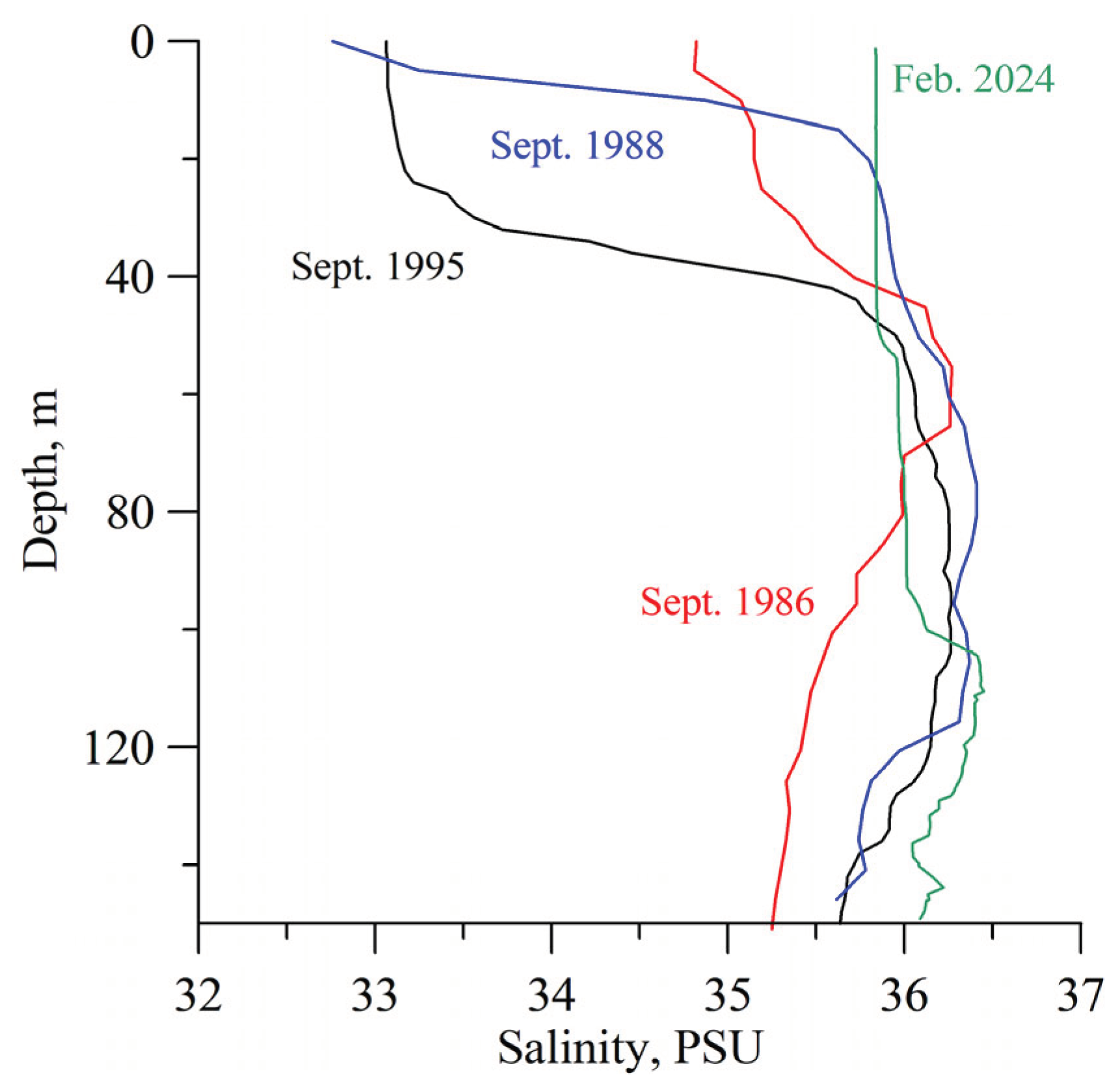
Individual CTD measurements sometimes reveal surface salinities lower than 33 PSU. Satellites estimate salinity only on the surface. The deep distribution of salinity in the plume shows that despite a decrease in surface salinity in September, the plume of desalinated waters is much shallower than in February (Figure 9 and Figure 10). A deeper plume core with less freshening is also detected. Such a core reaches depths of 100 m (Figure 10). Deep penetration of the cores depends on mixing during storms. We think that these two plumes are of different age and accordingly passed different distance to arrive to the location of measurements.
4. Discussion
The Amazon River discharges large amounts of freshwater into the ocean. This water gradually mixes with the surrounding seawater and spreads in the Atlantic transported by the North Brazil Current and later by the Northern Equatorial Current. As the plume spreads in the ocean, the storms mix the upper layer and low salinity water descends from the surface. At the same time water at the surface becomes less saline. Our section followed along 38°48ʹ W, whereas the Amazon delta is at 50° W. Thus, the direct distance from the Amazon delta exceeds 1200 km to reach the region of our measurements. Actually the distance is much longer, because first, the plume spreads to the northwest following the coastline, and only later turns to the east. During the propagation the water can be entrained into mesoscale eddies, which extend the traveled distance.
It is known from literature that the amount of freshwater discharge from the Amazon is subjected to strong seasonal variations. This causes pulses in spreading of the Amazon plume in the ocean, which is clearly seen on satellite images of surface salinity. The plume is best pronounced in the satellite images of surface salinity in August-December, which follows the maximum of the river’s discharge in June.
It follows from comparison of CTD sections made in April, September, and February (Figure 4, Figure 6, Figure 7, Figure 9) that in September the plume is located further north than in February and April. The more southern location of the plume after the period of maximum freshening may be associated with the separation of waters from the NECC current due to a series of anticyclonic eddies in the region of 40–30° W, arising between the NECC and sNEC, which is typical for the winter season [20].
Crossing of the plume in February shows a greater depth of desalination penetration and higher salinities in the plume than in September. The estimates of travel time from the river’s delta to the study site are about three months. The plume is best pronounced in September because it consists of water that left the delta region in June. The water that was recorded in February left the delta region approximately in November, the driest season. Our estimates based on Lagrangian modeling also indicate the travel time of the order of three months.
In addition, we think that the plume in February traveled a greater distance from the zone of direct influence of the Amazon River due to additional entrainment into the anticyclonic circulation separated from the NECC current, and could also be subject to greater influence of storms and mixing with surrounding ocean waters. Due to this, there was a greater deepening of the desalinated layer; and hence, an increase in salinity on the surface and throughout the plume layer.
5. Conclusions
Measurements of temperature and salinity in the Amazon River plume far from the river's mouth in the open ocean, with a resolution of 20 miles between stations, revealed the existence of the plume and its detailed structure. The connection with the Amazon River discharge was confirmed by the results of flow-through ship measurements of temperature and turbidity. Back in time Lagrangian analysis in the AVISO current velocity field showed that the source of fresh water in the measurement region is the Amazon.
Satellite observations of the plume allow us to study only its surface structure. The measurements allowed us to estimate the width of the Amazon plume core with salinity less than 36 PSU as 170 km, and the entire plume as 300–400 km. The desalination depth was from 50 to 100 m. Surface salinity decreased by 0.25 PSU compared to the background (36.1 PSU). Comparison with the measurements in other years in February showed a similar result for this month. Comparison with measurements in other months and especially in September, when the minimum salinity is usually recorded on the surface based on the satellite data, showed that the differences in salinity on the surface with the background salinity beyond the plume amounted to more than 3 PSU.
August–October is the period of maximum plume development, which is determined by satellite measurements of surface salinity. The Amazon discharge reaches its maximum in June after the rainy season. The spread of the plume to the area of our measurements in February takes about 3 months, during which waters of river origin are transported approximately over 3000 km. The extension of the transport path by approximately 700 km occurs due to additional anticyclonic circulation, which leads to the plume motion further to the east and then returning to the southwest. During this time, the plume water mixes with the surrounding waters by storms. Salinity in the plume decreases, and desalinization penetrates to greater depths.
Author Contributions
Conceptualization, E.M. and P.S.; methodology, E.M. and M.B., software, M.B.; validation, D.F.; formal analysis, E.M. and P.S.; data curation, D.F> and P.S.; writing—original draft preparation, E.M., P.S., and M.B.; writing—review and editing, E.M.; funding acquisition, E.M.; All authors have read and agreed to the published version of the manuscript.
Funding
This work was supported by the State Assignment of the Shirshov Institute of Oceanology (FMWE-2024-0016, ship measurements) and the Russian Science Foundation grant 21-77-20004 (analysis of measurement data), as well as by the State Assignments of the Pacific Oceanological Institute FEB RAS FWMM-2024-0032 (flow-through system data) and FWMM-2024-0014 (Lagrangian analysis).
Institutional Review Board Statement
Not applicable.
Informed Consent Statement
Not applicable.
Data Availability Statement
If needed to obtain the experimental information and data presented in the paper, please contact the author.
Acknowledgments
The authors thank the crew of R/V Akademik Mstislav Keldysh for the assistance in our scientific research.
Conflicts of Interest
The authors declare no conflicts of interest.
References
- Giffard, P., Llovel, W., Jouanno, J., Morvan, G., Decharme, D. Contribution of the Amazon River discharge to regional sea level in the tropical Atlantic Ocean, Water, 2019, 11(11), 2348. [CrossRef]
- Dai, A., Trenberth, K.E. Estimates of freshwater discharge from continents: latitudinal and seasonal variations. J. Hydrometeorol., 2002, 3, 660–687. [CrossRef]
- Liang, Y.-C., Lo, M.-H., Lan, C.-W., Seo, H., Ummenhofer, C.C., Yeager, S., Wu, R.-J., Steffen, J.D. Amplified seasonal cycle in hydroclimate over the Amazon river basin and its plume region. Nat. Commun., 2020, 11, 4390. [CrossRef]
- Varona, H.L., Veleda, D., Silva, M., Cintra, M., Araujo, M. Amazon River plume influence on Western Tropical Atlantic dynamic variability, Dynamics of Atmospheres and Oceans, 2019, 85, 1–15. [CrossRef]
- Müller-Krager, F.E., McClain, C.R., Richardson, P.L. The dispersal of the Amazons water. Nature, 1988, 333, 56–59. [CrossRef]
- Jo, Y.-H., Yan, X.-H., Dzwonkowski B., Liu W.T. A study of the freshwater discharge from the Amazon River into the tropical Atlantic using multi-sensor data, Geophys. Res. Lett., 2005, 32, L02605. [CrossRef]
- Cooley, S.R., Coles, V.J., Subramaniam, A., Yager, P.L. Seasonal variations in the Amazon plume-related atmospheric carbon sink, Global Biogeochem. Cycles,2007, 21, GB3014. [CrossRef]
- Hu, C., Montgomery, E.T., Schmitt, R.W., The dispersal of the Amazon and Orinoco River water in the tropical Atlantic and Caribbean Sea: Observation from space and S-PALACE floats. Deep Sea Research Part II, 2004, 51, (10–11), 1151–1171. [CrossRef]
- Coles, V.J., Brooks, M.T., Hopkins, J., Stukel, M.R., Yager, P.L., Hood, R.R. The pathways and properties of the Amazon River plume in the tropical North Atlantic Ocean, J. Geophys. Res. Oceans, 2013, 118, 6894–6913. [CrossRef]
- Gouveia, N.A., Gherardi, D.F.M., Aragão, L.E.O.C. The role of the Amazon River plume on the intensification of the hydrological cycle. Geophysical Research Letters. 2019, 46, 12,229–12,221. [CrossRef]
- Korosov, A., Counillon, F., Johannessen, J.A. Monitoring the spreading of the Amazon freshwater plume by MODIS, SMOS, Aquarius, and TOPAZ, J. Geophys. Res.Oceans, 2015, 120, 268–283. [CrossRef]
- Morozov, E.G., Zavialov, P.O., Zamshin, V.V., Moller, O.O. Jr., Frey, D.I., Zuev, O.A., Seliverstova, A.M., Chultsova, A.L., Bulanov, A.V., Lipinskaya, N.A., Krechik, V.A., Chvertkova, O.I. Mixing zone between the Amazon River plume and open ocean, Russian J. Earth Sciences, 2023, 23, ES4006. [CrossRef]
- Fratantoni, D.M., Richardson, P.L. The evolution and demise of North Brazil Current rings, J. Phys. Oceanogr., 2006, 36, 1241–1264.
- Prants, S.V. (2015), Backward-in-time methods to simulate large-scale transport and mixing in the ocean. Phys. Scr., 2015, 90, 074054. [CrossRef]
- Budyansky, M.V., Udalov, A.A., Lebedeva, M.A., Belonenko, T.V. Assessment of pollution of the waters in the South Kuril Fishing Zone of Russia by radioactive waters from the Fukushima-1 NPP based on Lagrangian Modeling, Doklady Earth Sciences, 2024. [CrossRef]
- Budyansky, M.V., Goryachev, V.A., Kaplunenko, D.D., Lobanov, V.B., Prants, S.V., Sergeev, A.F., Shlyk, N.V., Uleysky, M.Yu., Role of mesoscale eddies in transport of Fukushima-derived cesium isotopes in the ocean, Deep Sea Research Part I, 2015, 96, 15–27. (submitted; accepted; in press). [CrossRef]
- Fayman, P.A., Salyuk, P.A., Budyansky, M.V., Burenin, A.V., Didov, A.A., Lipinskaya, N.A., Ponomarev, V.I., Udalov, A.A., Morgunov, Y.N., Uleysky, M.Y., et al. Transport of the Tumen River Water to the Far Eastern Marine Reserve (Posyet Bay) Based on in Situ, Satellite Data and Lagrangian Modeling Using ROMS Current Velocity Output. Mar. Pollut. Bull., 2023, 194, 115414. [CrossRef]
- Boyer, T.P., Baranova, O.K., Coleman, C., Garcia, H.E., Grodsky, A., Locarnini, R.A., Mishonov, A.V., Paver, C.R., Reagan, J.R., Seidov, D., Smolyar, I.V., Weathers, K., Zweng, M.M. World Ocean Database 2018. Mishonov A.V., Technical Ed., NOAA Atlas NESDIS 87.
- Fore, A., Yueh, S., Tang, W., Hayashi, A., SMAP Salinity and Wind Speed Data User’s Guide, Version 3.0. Jet Propulsion Laboratory, California Institute of Technology, 2016.
- Dimoune, D.M., Birol, F., Hernandez, F., Léger, F., Araujo, M.: Revisiting the tropical Atlantic western boundary circulation from a 25-year time series of satellite altimetry data, Ocean Sci., 2023, 19, 251–268. [CrossRef]
Figure 1.
Map of surface salinity based on satellite data.
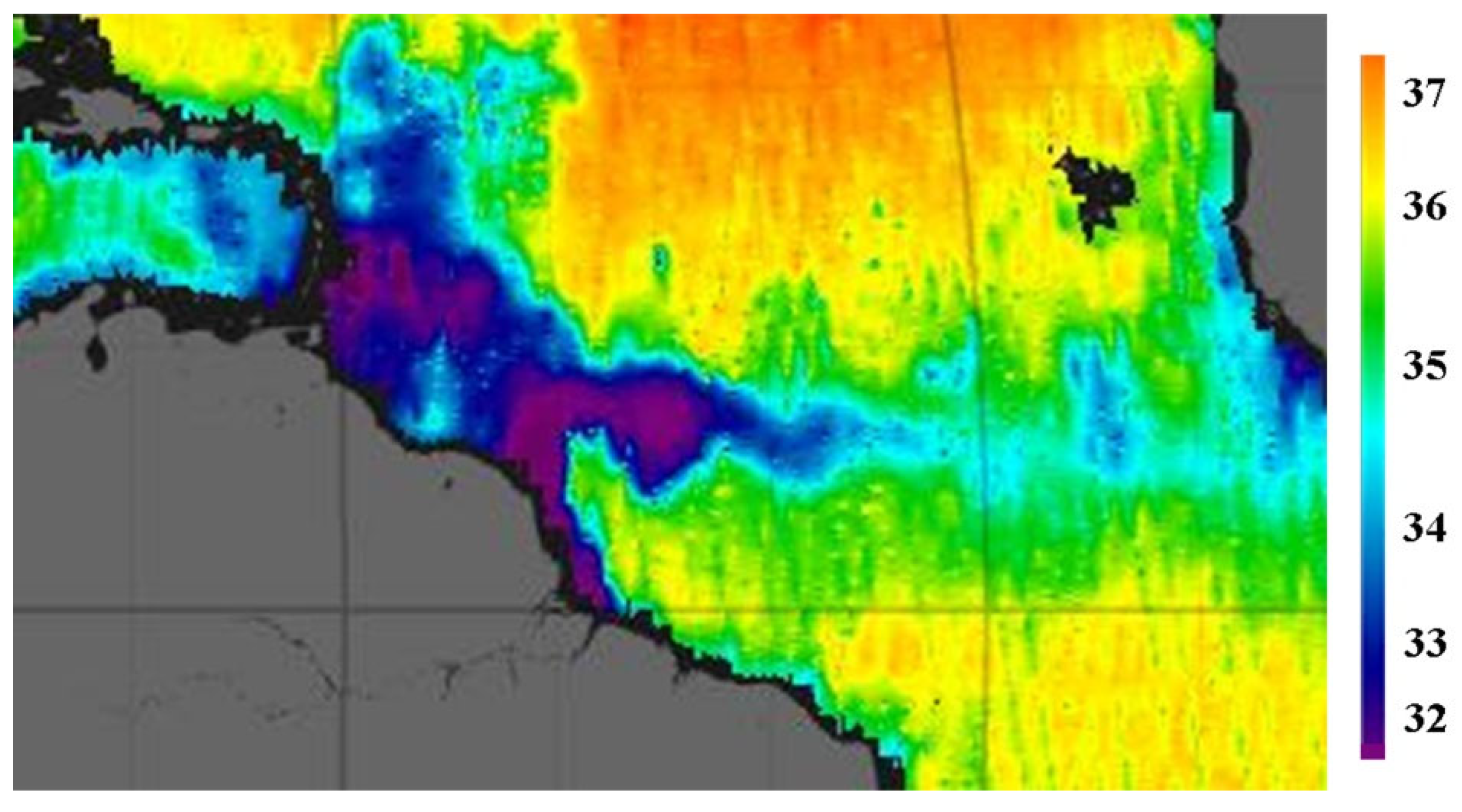
Figure 2.
Scheme of currents in the western tropical Atlantic that transport Amazon River waters in the ocean [13].
Figure 2.
Scheme of currents in the western tropical Atlantic that transport Amazon River waters in the ocean [13].
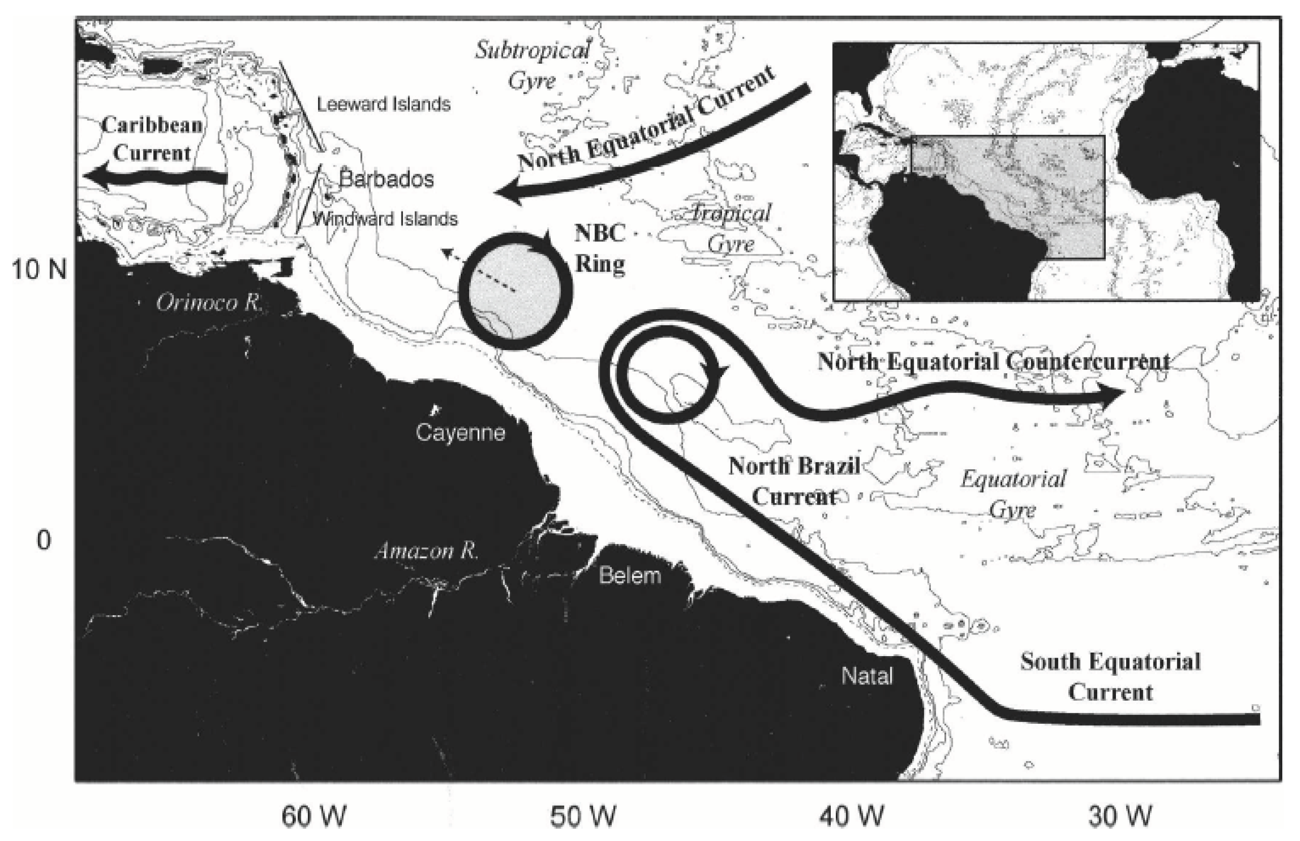
Figure 3.
Absolute dynamic topography of the tropical West Atlantic on February 26, 2024.
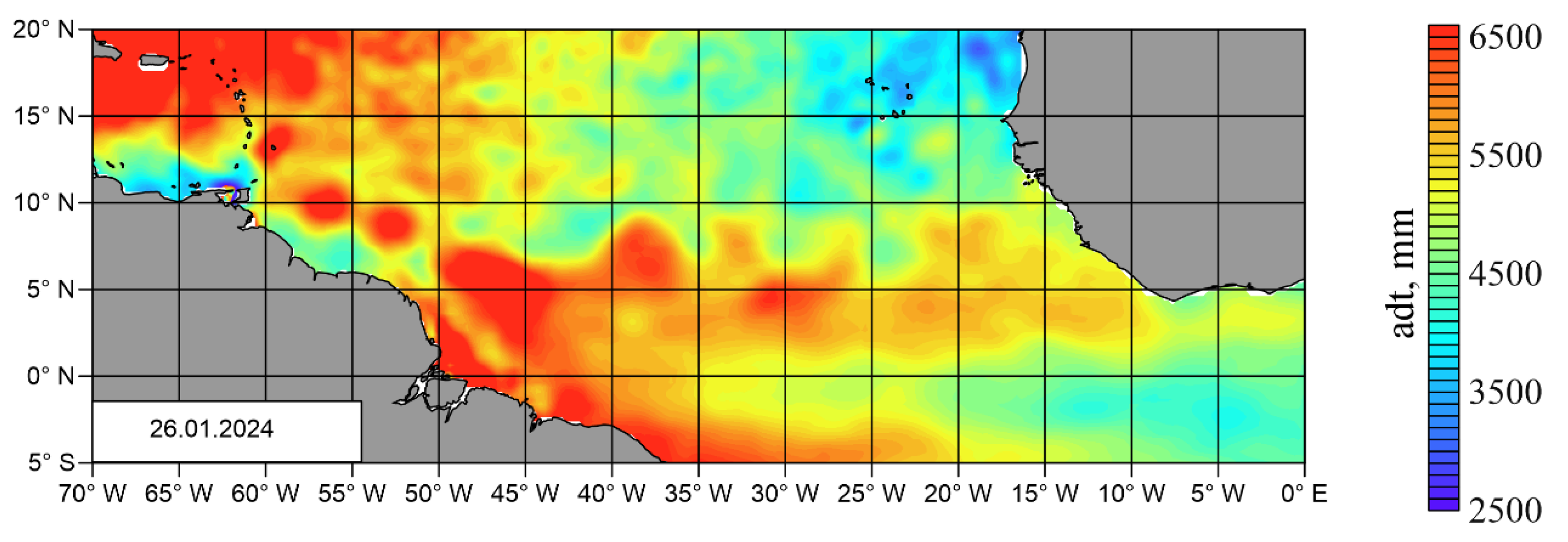
Figure 4.
Salinity section at the intersection with the plume of desalinated waters at 38°48.0ʹ W on February 1–2, 2024 (left top panel). Salinity profile at the station at latitude 5°20ʹ N (right top panel). Graphs of changes in salinity and turbidity as recorded by the vessel's flow system (bottom panel).
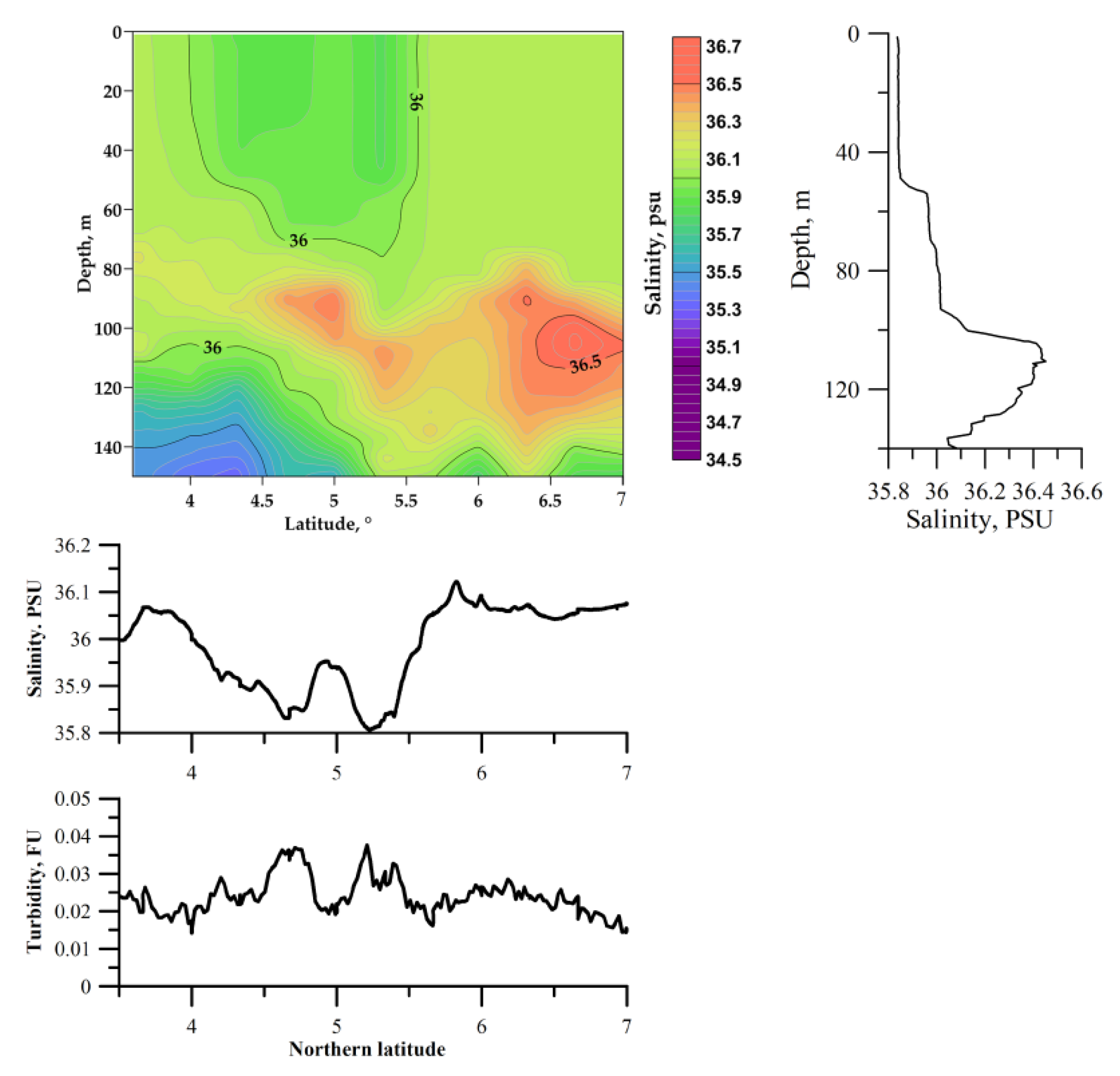
Figure 5.
Composition of daily traces of trajectories of passive markers simulating Amazon waters, selected in the segment with the minimum measured salinities (5°12.0ʹ –5°15.6ʹ N, 38°48ʹ W). The marker trajectories were calculated back in time over 180 days based on the AVISO velocity field. Trajectories were truncated south of 3° N because geostrophic approximation is not valid close to the equator.
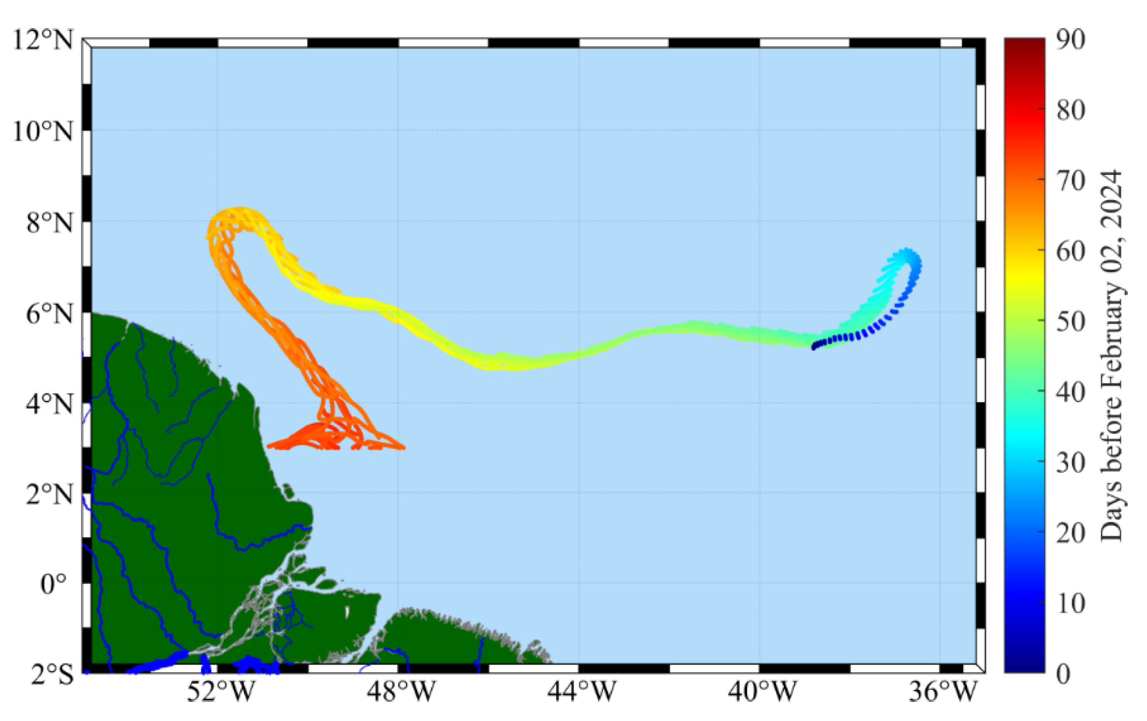
Figure 6.
Salinity section when crossing a plume of desalinated waters at 35°00ʹ W on April 27–29, 1996.
Figure 6.
Salinity section when crossing a plume of desalinated waters at 35°00ʹ W on April 27–29, 1996.
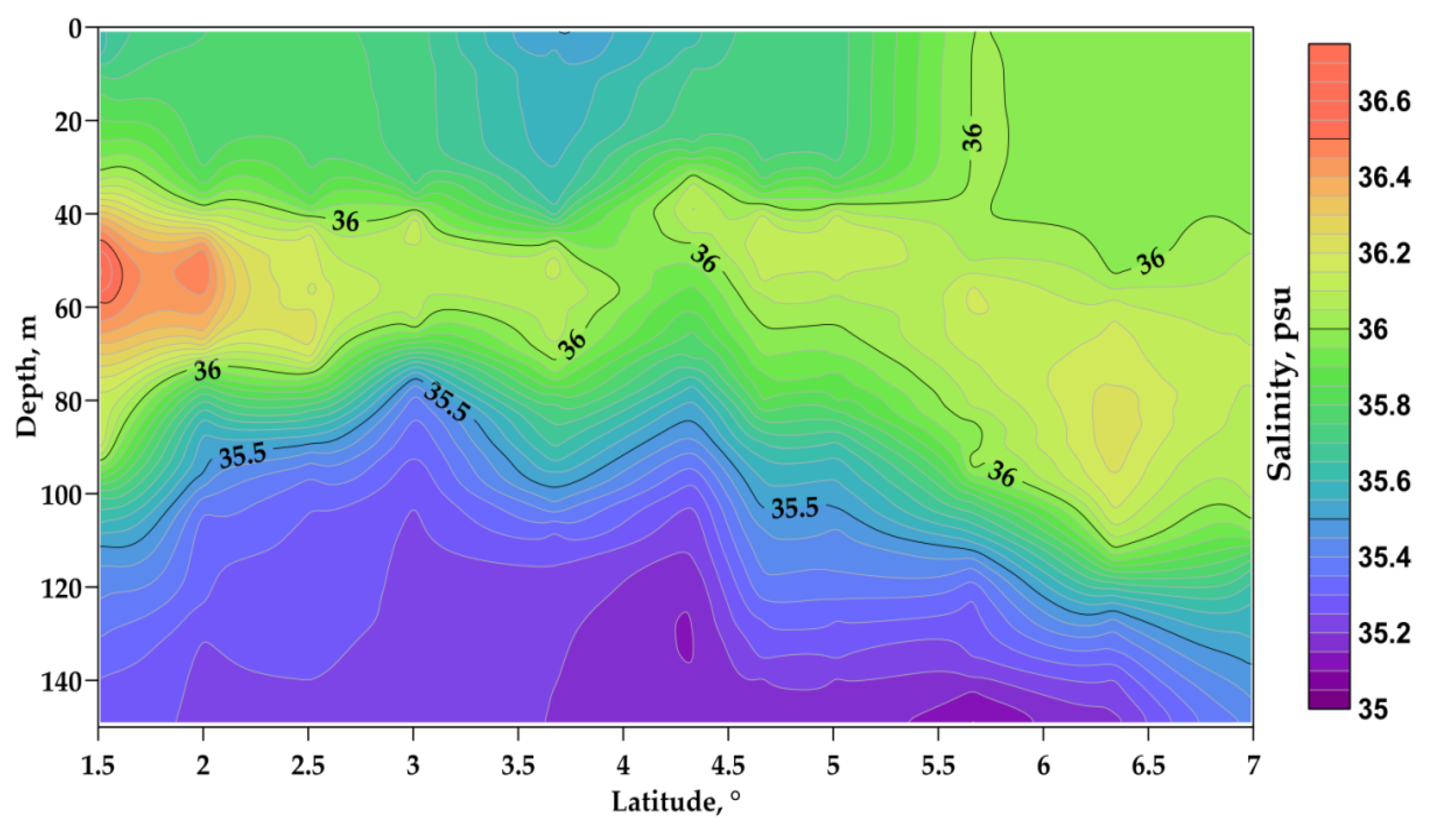
Figure 7.
Salinity section when crossing a plume of desalinated waters at 35°00ʹ W on February 4–5, 1993.
Figure 7.
Salinity section when crossing a plume of desalinated waters at 35°00ʹ W on February 4–5, 1993.
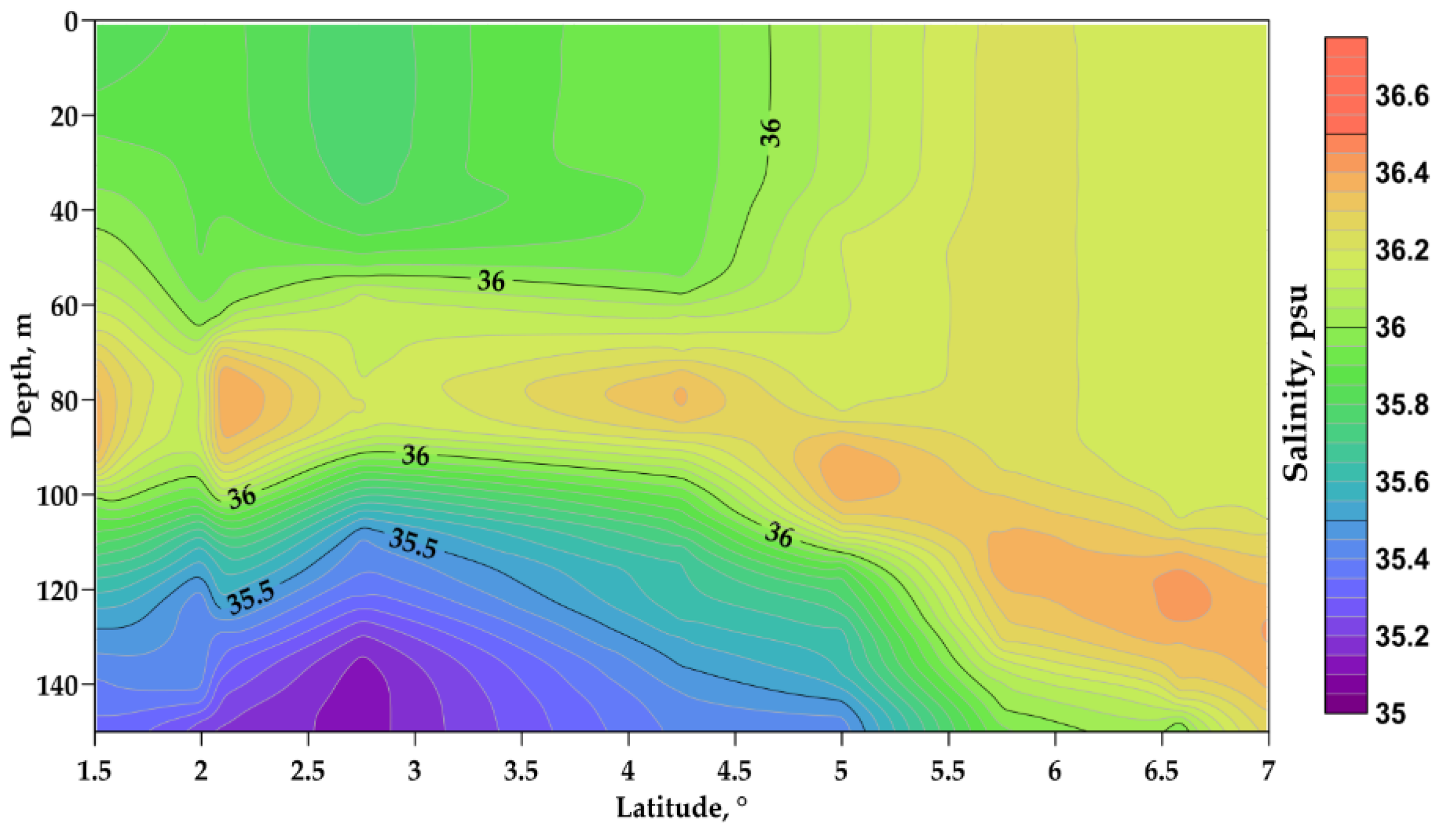
Figure 8.
Intra-annual variations in the surface salinity of the Amazon plume based on the SMAP satellite data in 2019 [12,19].
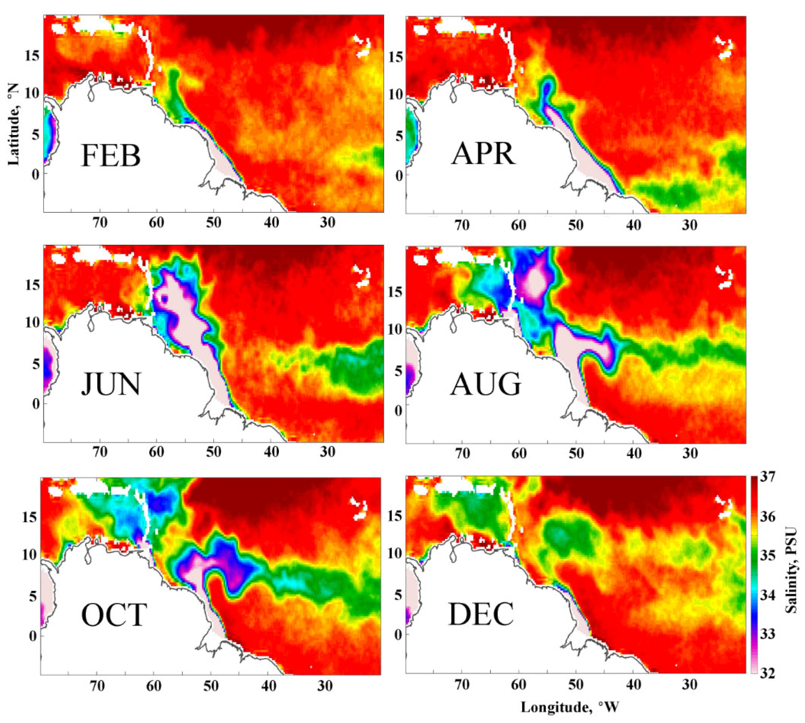
Figure 9.
Salinity section when crossing a plume of desalinated waters at 34°00ʹ W on September 3–5, 1986.
Figure 9.
Salinity section when crossing a plume of desalinated waters at 34°00ʹ W on September 3–5, 1986.
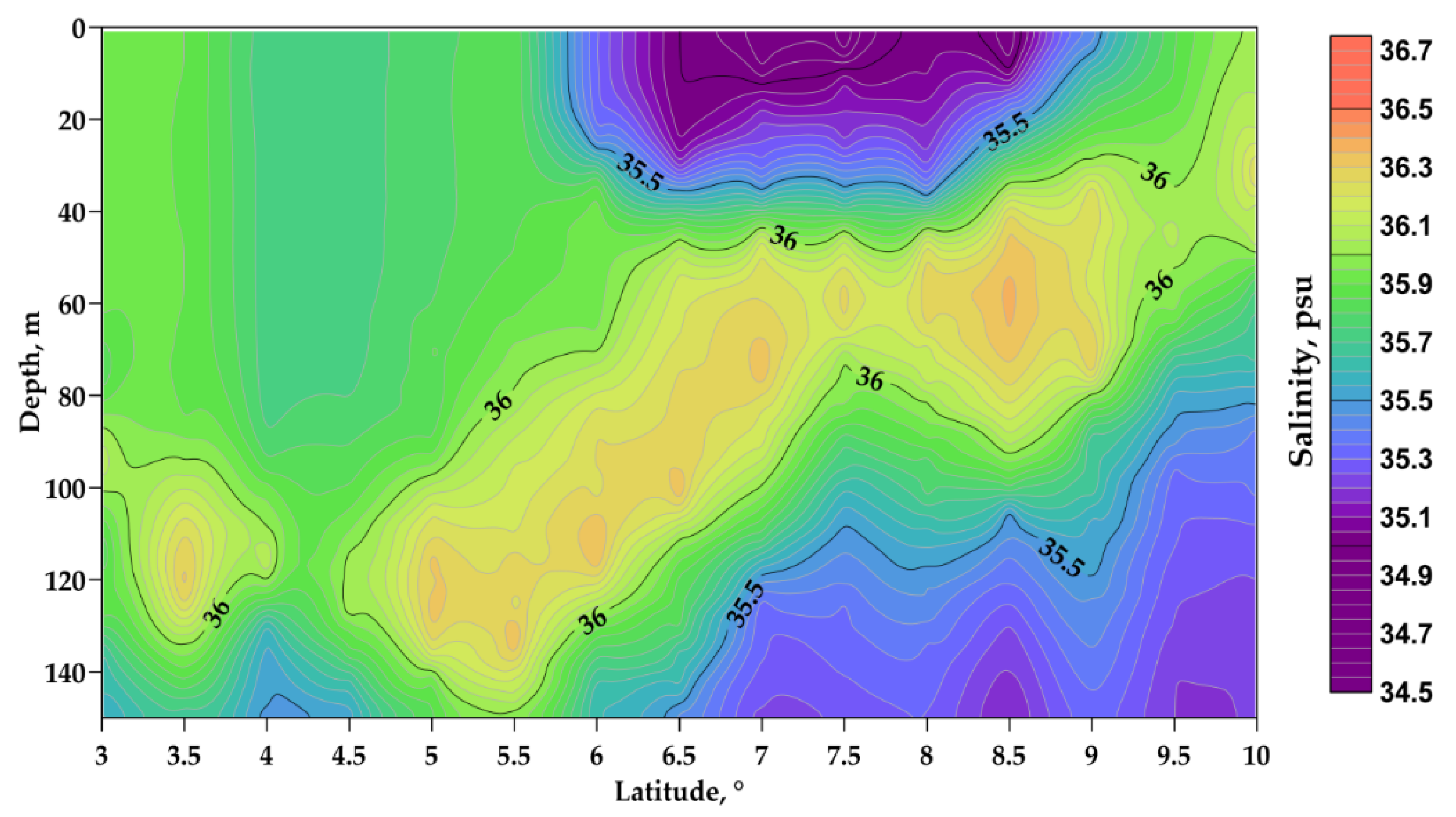
Figure 10.
Vertical distributions of salinity in September during the period of minimum salinity on the surface in different years in comparison with our data in February 2024.
Figure 10.
Vertical distributions of salinity in September during the period of minimum salinity on the surface in different years in comparison with our data in February 2024.
Disclaimer/Publisher’s Note: The statements, opinions and data contained in all publications are solely those of the individual author(s) and contributor(s) and not of MDPI and/or the editor(s). MDPI and/or the editor(s) disclaim responsibility for any injury to people or property resulting from any ideas, methods, instructions or products referred to in the content. |
© 2024 by the authors. Licensee MDPI, Basel, Switzerland. This article is an open access article distributed under the terms and conditions of the Creative Commons Attribution (CC BY) license (http://creativecommons.org/licenses/by/4.0/).
Copyright: This open access article is published under a Creative Commons CC BY 4.0 license, which permit the free download, distribution, and reuse, provided that the author and preprint are cited in any reuse.


